Vectors

Topics covered in this section are:

1. Introduction
   1. Scalars
   2. Vectors
2. Addition of Vectors
   1. Triangle Law
   2. Parallelogram Law
   3. Magnitude and Direction of Resultant
   4. Difference of two Vectors
3. Representation of vectors
   1. Vectors on coordinate plane
   2. Vectors in 3-dimensional space
   3. Addition of vectors in component form
   4. Negation of vector in component form

1. Introduction

In our everyday-life, we encounter three quantities - Scalars, Vectors and Higher rank Tensors. To say, Scalar and Vectors are zero and 1st rank tensors, respectively. But, we won't be discussing higher rank tensors here.

• Scalars:

Definition: Scalars are the quantities which have only magnitudes but no direction.
For example, distance, speed, charge, volume, mass, numbers etc.

Now, we can perform additon, subtraction, multiplication and divison on the scalars in the same way we perform these operations on numbers (algebriac operations). Let us consider two scalar values, say \(5C\) and \(-1C\) of charges, where \(C\) is Coulomb.

If they are put together, then we say that \((5-1)C= 4C\), of charge is at that place. Similarly, other operations are performed.




• Vectors:

Definition: Vectors are any physical quantity which have direction as well as magnitude.
For example, displacement, velocity, force, angular speed, etc.

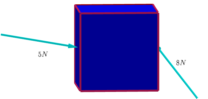
Let's take the example of force. When we push an object with a force, we can feel how hard we are pushing it. This is in a sense a measure of magnitude of the force. Further, we can push the object from different directions as shown in Figure 1.1, this is the direction of the force.



Vectors are denoted by a boldface letter such as \(\textbf{A}\) or with an arrow on head of the letter i.e. as \(\vec{A}\). We would take up the arrow on head notation in rest of the discussion. In diagrams, we represent vectors using arrows, such that its magnitude (denoted as \(|\vec{A}|\) or simply \(A\)) is proportional to the length of arrow and direction indicated by the head of the arrow. This can be seen in the Figure 1.1.



• Equal vectors and Opposite/ Negative Vectors:

Two vectors \(\vec{A}\) and \(\vec{B}\) are said to be equal iff the have they same magnitude as well as direction, as shown in Figure 1.2.



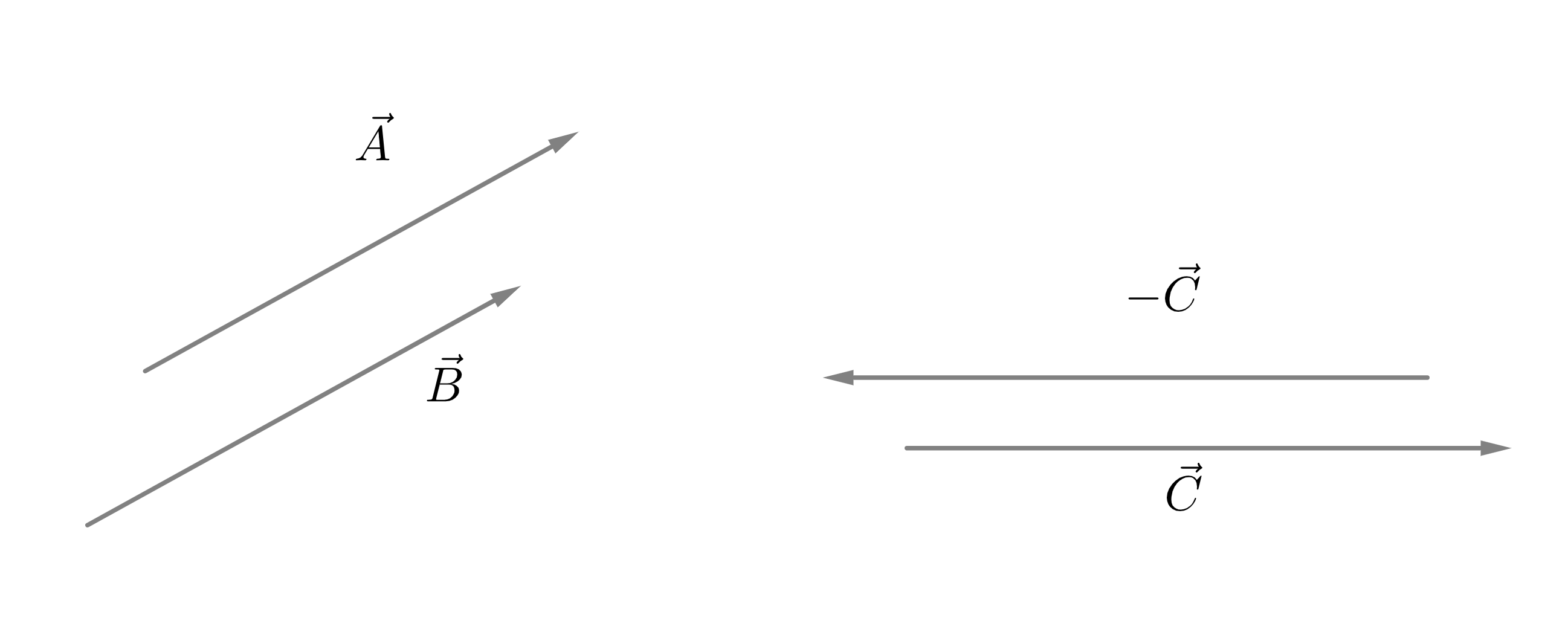
And, one vector is said to be opposite of other vector, say \(\vec{C}\) or the negative of that vector iff they have the same magnitude but point in opposite directions and is denoted as \(-\vec{C}\). This is also shown in Figure 1.2.

But, the arithmetic operations on the vectors doesn't operate in the normal algebriac way. We now move to discuss these operations in detail.

2. Addition of Vectors

Additon of two vectors is performed using two laws:

1. Triangle Law:



Consider the vectors \(\vec{A}\) and \(\vec{B}\) as shown in Figure 2.1. When, the three vectors \(\vec{A}\), \(\vec{B}\) and \(\vec{R}\) forms a triangle with the tail of \(\vec{B}\) on the head of \(\vec{A}\), the traingle law of vector addition can be stated as :

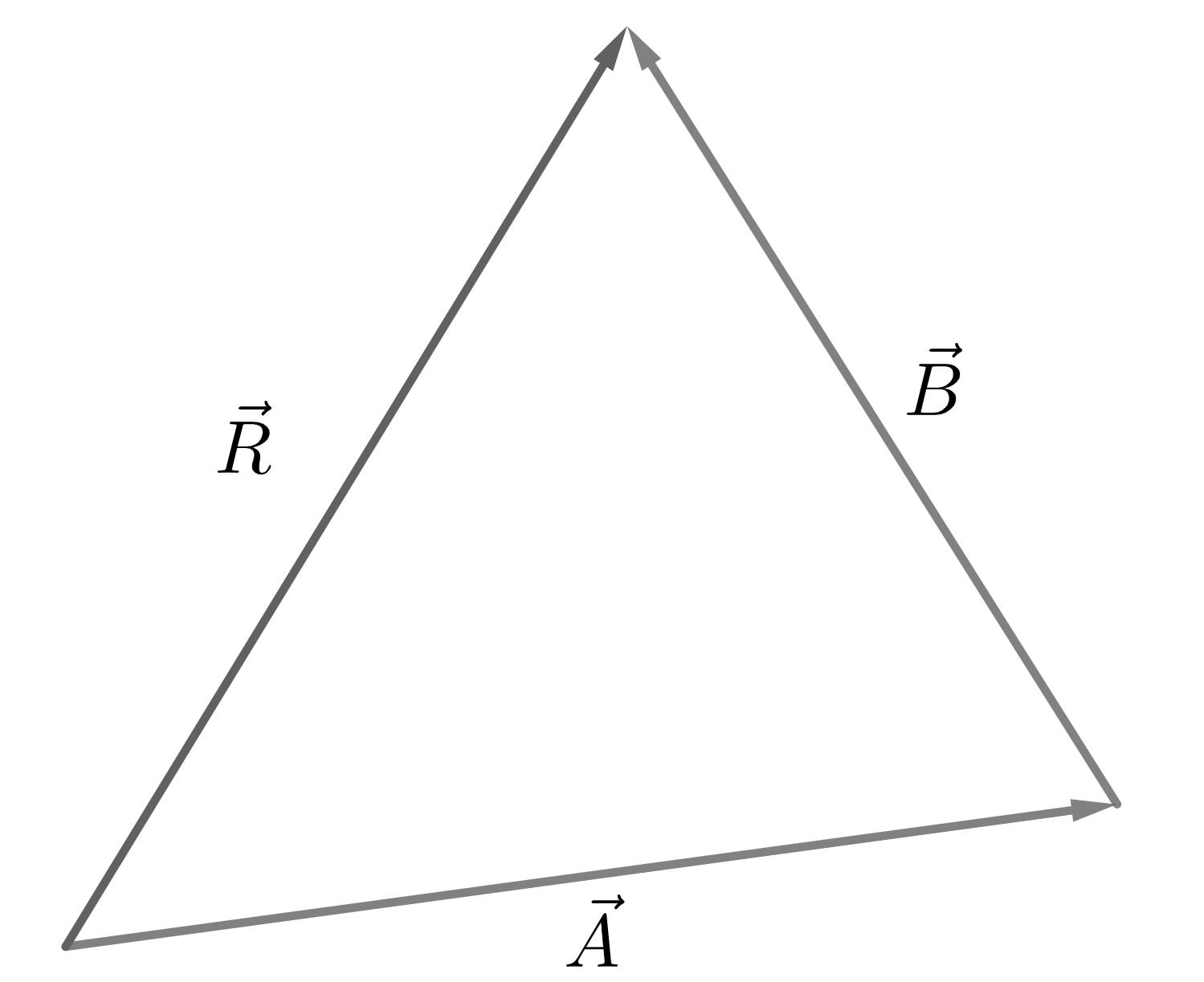
The resultant (or sum of) the vectors \(\vec{A}\) and \(\vec{B}\), \(\vec{R}\) is the vector from the the tail of \(\vec{A}\) to the head of \(\vec{B}\).

This is known as Triangle law of vector addition as the three vectors involved are forming a triangle for the rule to apply.



Example:



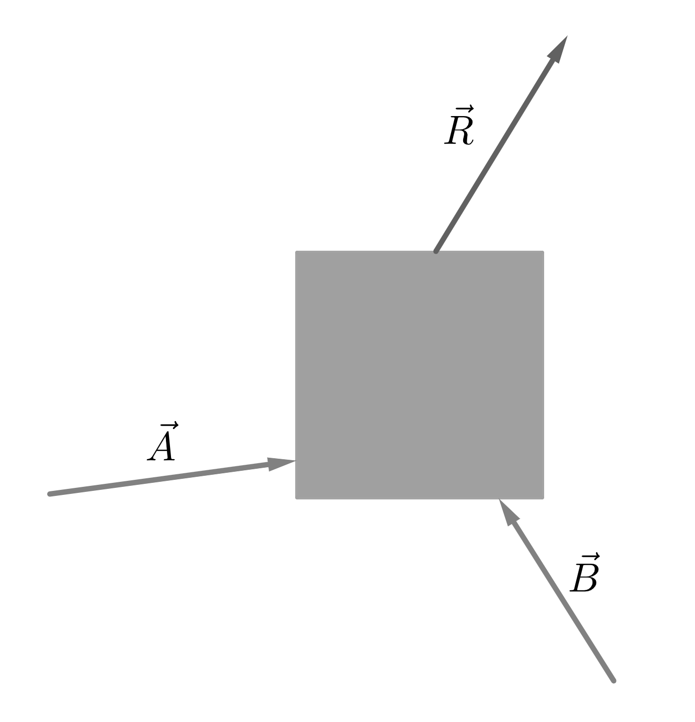
If we apply force \(\vec{A}\) and \(\vec{B}\) on a plate as shown in Figure 2.2, then the plate would have a net motion in the direction of \(\vec{R}\) as shown. This is the insight over the triangle law. One may notice that the vectors are pararllelly translated and then made into triangle of Figure 2.1. This shows that the vectors, irrespective of their position in space, represent the exactly same thing as long as their magnitude and direction are the same.







2. Parallelogram Law:

Again, consider the vectors \(\vec{A}\) and \(\vec{B}\) arranged (by parallel translation) such that the tail of \(\vec{A}\) and \(\vec{B}\) coincides. Now, the parallelogram law can be stated as follows:



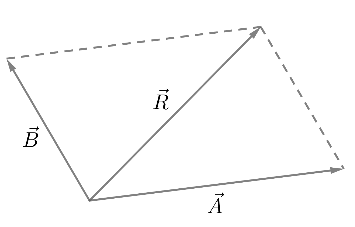
The resultant or the sum of two vectors, \(\vec{A}\) and \(\vec{B}\) is the diagonal of the parallelogram formed by \(\vec{A}\) and \(\vec{B}\) as adjacent sides, directed from the point of coincidence of tail of the two vectors to the opposite vertex of the parallelogram i.e. the vector \(\vec{R}\) in the Figure 2.3.

This is the same as the Triangle law as we can parallelly translate the vector \(\vec{B}\) to the right side of the paralleogram and form the triangle as was in the Figure 2.1. But, the two of them have their own significance as we use Parallelogram law to find the magnitude of resultant vector and triangle law in expressing one vector as difference of two, to say one of many uses.

Example :



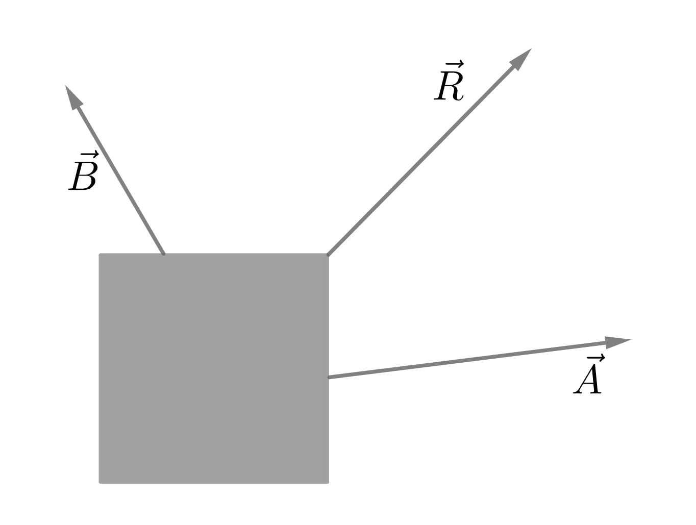
Consider the Figure 2.4 as shown. It is just a reimagination of the Triangle Law Example using the Paralellogram Law. Some may find this one more intuitive as the forces \(\vec{A}\) and \(\vec{B}\) are shown so as to form a parallelogram, imagining the forces to be pull forces instead of push forces as was in the Figure 2.2. These eamples illustrates the variety of methods, each having their own beauty, to analyse a given situation.

We now move towards quantifying the above analysis.

• Magnitude and direction of Resultant vector:

Consider two vectors \(\vec{a}\) and \(\vec{b}\) (with magnitudes \(a\) and \(b\) respectively), with an angle \(\theta\) between the two vectors, when they are joined tail to tail, as shown in the Figure 2.5.
It can be noted that whenever we say angle between two vectors, we talk about this angle only (i.e. when they are joined tail to tail.)



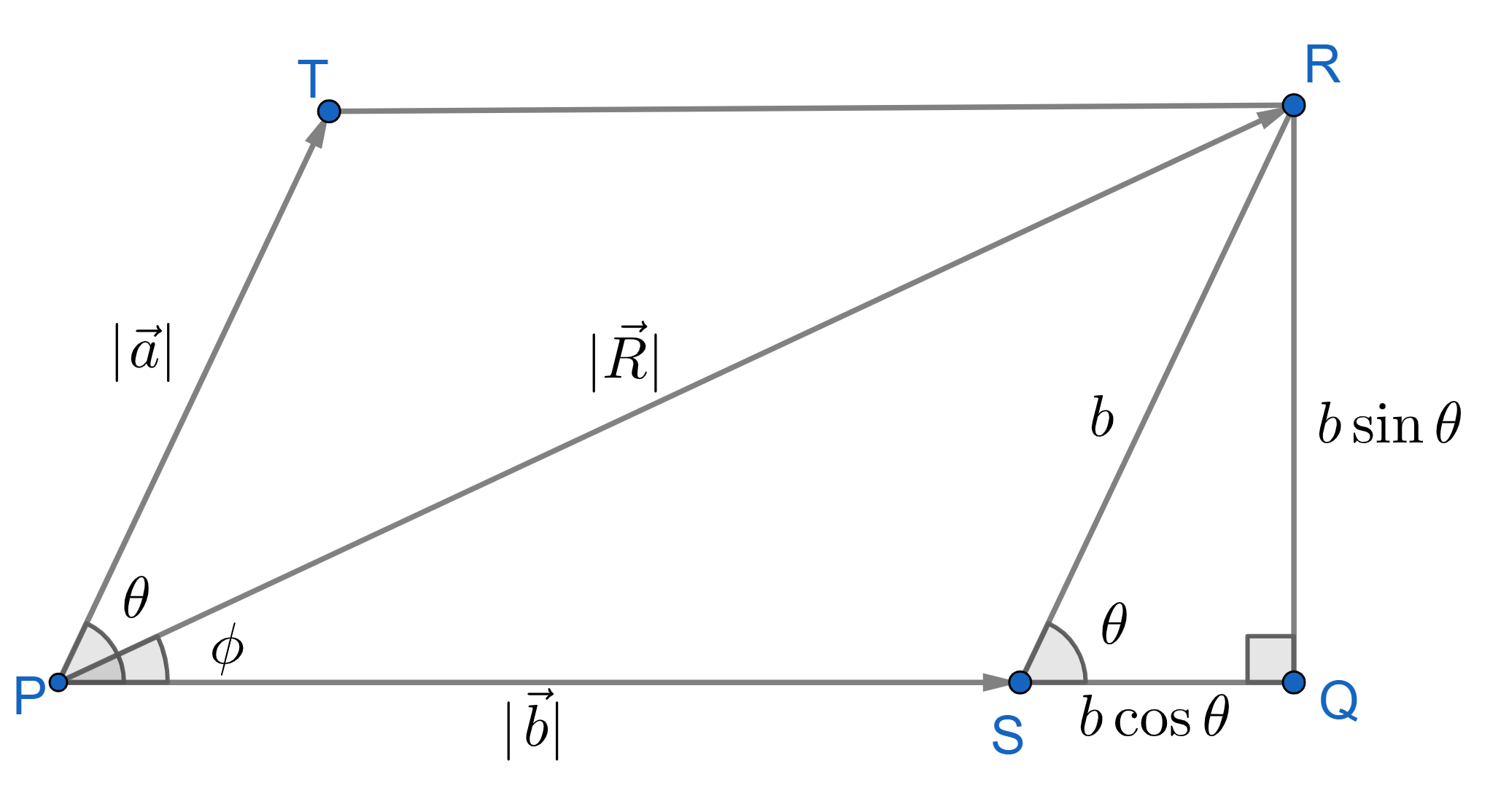
Using parallelogram law, we can draw the parallelogram \(PSRT\) and assign the diagonal \(PQ\) as the resultant vector \(\vec{R}\). Also, \(SR = PT = b\). Further, using simple trigonometry, we get the side lengths of the right angled triangle, \(\triangle RQS\) as : $$ \begin{align} SQ &= b\cos{\theta} \\ RQ &= b\sin{\theta} \end{align} $$

Now, from the right angled triangle \(\triangle PQR\) and using pythagoras theorem,

$$ \begin{align} |R|^2 &= (a+b\cos{\theta})^2 + (b\sin{\theta})^2 \\ \implies R^2 &= a^2+ b^2 \cos^2{\theta} + 2ab\cos{\theta} + b^2\sin^2{\theta} \\ \implies R &= \sqrt{a^2+b^2 + 2ab\cos{\theta}}\hspace{1cm} \color{red}{(2.1)} \end{align} $$ In the last step we used the identity, \(\sin^2{\theta} + \cos^2{\theta} = 1\). Equation 2.1 gives the magnitude of the resultant of two vectors described above.

Now, for the direction of the resultant vector, say it is at an angle \(\phi\) with the vector \(\vec{a}\) as shown in Figure 2.5. Then, from \(\triangle PQR\), we get: $$ \begin{align} \tan{\phi} &= \frac{QR}{PQ} = \frac{b\sin{\theta}}{a+b\cos{\theta}} \\ \implies \phi &= \tan^{-1}\left(\frac{b\sin{\theta}}{a+b\cos{\theta}}\right) \hspace{1cm} \color{red}{(2.2)} \end{align} $$

Special Case\(\left(|\vec{a}|=|\vec{b}|\right)\): When the two vectors \(\vec{a}\) and \(\vec{b}\) have the same length, say \(a\) and angle between them be \(\theta\). Then, using equation 2.1, the resultant would have magnitude as: $$ \begin{align} R &= \sqrt{a^2 + a^2 + 2a^2 \cos{\theta}}\\ \implies R &= \sqrt{2a^2(1+\cos{\theta})}\\ \implies R &= \sqrt{2a^2\times 2\cos^2{\left(\frac{\theta}{2}\right)}}\\ \implies R &= 2a\cos{\left(\frac{\theta}{2}\right)} \hspace{1cm} \color{red}{(2.3)} \end{align} $$ In this case, the resultant vector would be along the angle bisector of between the two vectors i.e. \(\phi=\frac{\theta}{2}\).




• Difference of two vectors:

The difference of two vectors is the sum of the first vector and the negative of the vector being subtracted. Consider the same vectors \(\vec{a}\) and \(\vec{b}\) again as shown in Figure 2.6.



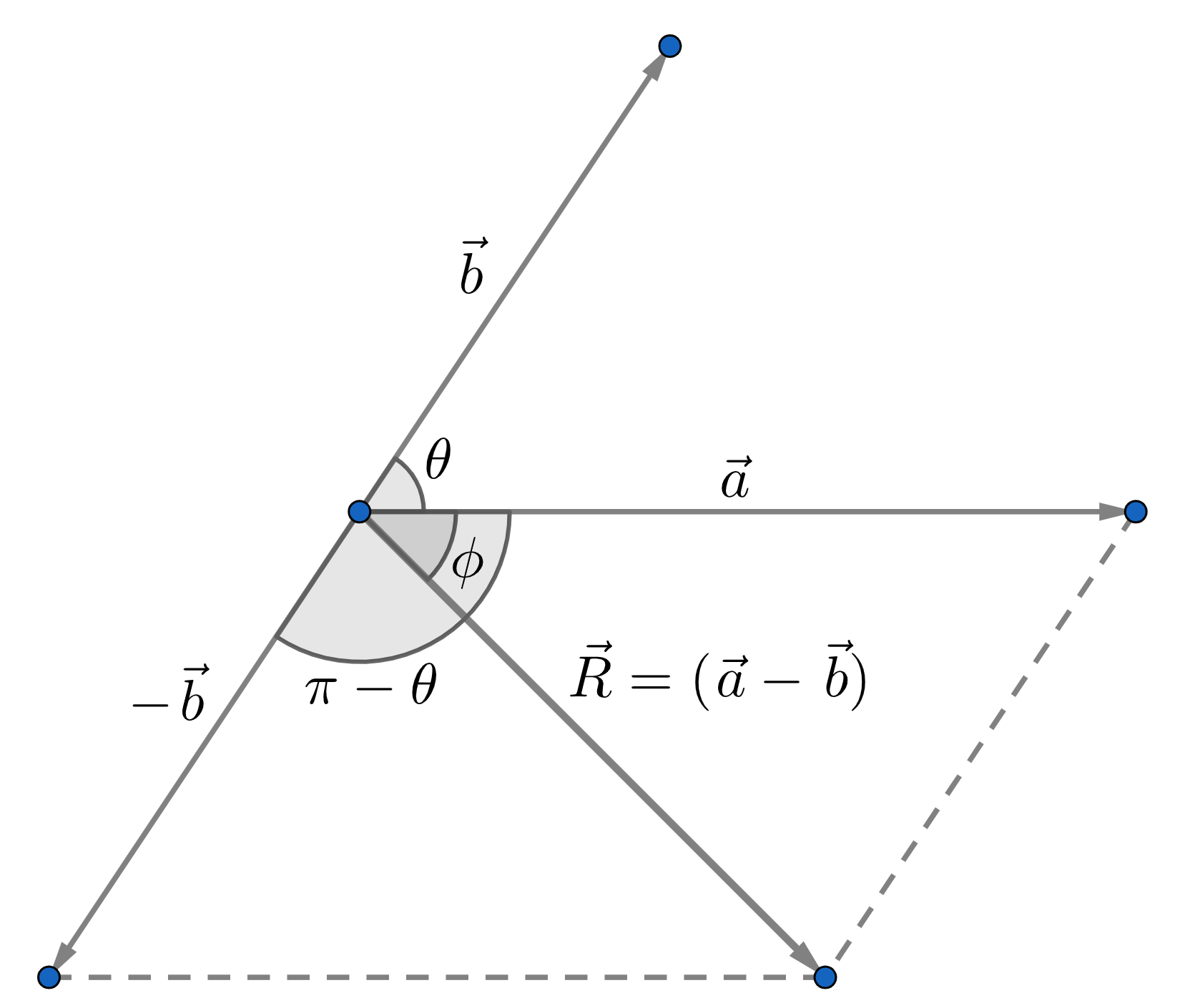
We have to find the difference \(\vec{a}-\vec{b}\). So, we rewrite it as \((\vec{a}+(-\vec{b}))\). And clearly, this represents the diagonal of the parallelogram formed by \(\vec{a}\) and \(-\vec{b}\) as its resultant, as shown in figure.

Since, here the angle between \(\vec{a}\) and \(\vec{b}\) is \(\theta\), so the angle between \(\vec{a}\) and \(-\vec{b}\) (the vectors which originally have to be "added") would be \((\pi-\theta)\). Now, using the equation 2.1 for the magnitude of \(\vec{R}\), we get:

The magnitude of the resultant vector after subtracting the two vectors:

$$ \begin{align} |\vec{R}| = |\vec{a}-\vec{b}| &= \sqrt{a^2 + b^2 + 2ab \cos(\pi-\theta)} \\ R &= \sqrt{a^2 + b^2 - 2ab\cos\theta}\\ (\because \cos(\pi-\theta) &= -\cos{\theta}) \end{align} $$

If you have noticed, we have taken the magnitude of the negative vector, \(-\vec{b}\) to be the same \(b\). This is because the length of the vector remains the same even after negating it. The angle \(\phi\) that gives the direction of \(\vec{R}\) is calculated in the same way as is done above.

3. Representation of vectors

Vectors are represented in many different ways, primarily depending on the use and context of use. One of the representation has been discussed in the starting of this section, the arrow representation.

Here we would be describing yet another representation, which is very useful primarily in Physics, the basis vector representation /component form of a vector. This representation makes many operations on vectors easy to be computed and visualized.

• Vectors on coordinate plane:

Consider a point in the \(2\)-dimensional plane, \((x, y)\). Also, consider an arrow pointing from the origin to this point as shown in Figure 3.1.



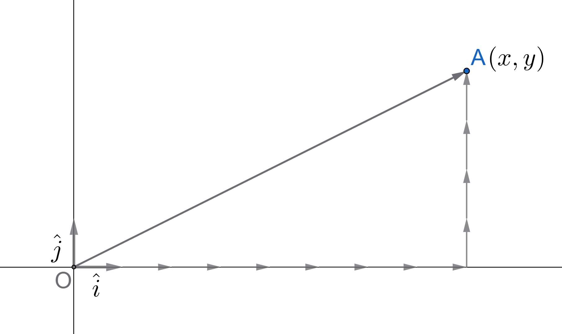
Considering the arrow to be a vector (say, \(\vec{A}\)). From figure, we can see that the vector \(\vec{A}\) can be can be formed by adding multiples of two other vectors, one along each of the \(x\) and \(y\)-axes. This is just the result of triangle law of vector addition. In the particular case shown, the vector \(\vec{A}\) is made from \(8\) vectors along \(x\)-axis and \(4\) vectors along \(y\) axis.

Anyway, we can genralize it to be \(x\) vectors along the \(x\)-axis and \(y\) vectors along the \(y\)-axis. The two vectors are known as Basis vectors for \(2D\) plane and are denoted as \(\hat{i}\) (or \(\hat{x}\)) for basis along \(x\)-axis and \(\hat{j}\) (or \(\hat{y}\)) for that along \(y\)-axis (see figure).




• Standard basis in \(2D\):

Till now, we have been talking of the basis vectors as abstract objects and haven't quantified them yet. In \(2D\), basis can be any two vectors pointing in different directions (for datails, see Linear Algebra on Math Derived). But to make the calculations easy and to maintain some standard of vector representation, we have defined the basis as:

• \(\hat{i}\) : The vector representing the arrow from the origin, \((0, 0)\) to the point \((1, 0)\) in the \(xy\)-plane.
• \(\hat{j}\) : The vector representing the arrow from the origin, \((0, 0)\) to the point \((0, 1)\) in the \(xy\)-plane.
These are known as the Standard basis in two dimensions, refer the Figure 3.1. See Unit vector below for the symbol.

Let's write down the above vector \(\vec{A}\) in this representation, using the standard basis. In this representation, the vector is written as the sum of multiples (as much as used in making the vector) of the basis vectors. This makes the calculation very easy and intuitive as we will see shortly. So, the vector \(\vec{A}\) is: $$ \vec{A} = 8\hat{i} + 4\hat{j} $$

This is for the particular vector going from the origin to the point \((8, 4)\). For any general vector from origin to point \((x, y)\), the representation gives: $$ \boxed{\vec{A} = x\hat{i} + y\hat{j}} \hspace{1cm} \color{red}{(3.1)} $$

This representation is known as the basis vector representation since we are writing the vector in terms of the basis vectors. Further, it is known as the component form since the components of a particular vector about the axes is explicitly shown in this represenatation. Here, the components of \(\vec{A}\) are \(x\) about the \(x\)-axis and \(y\) about the \(y\)-axis.



• Vectors in 3-dimensional space:



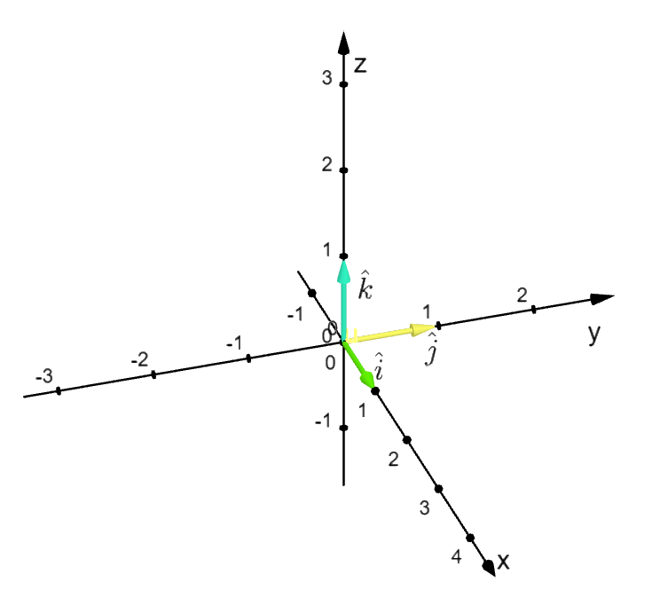
The above analysis can be easily generalized to three dimensions. We consider a vector (in arrow form, say \(\vec{A}\)) from the origin, \((0, 0, 0)\) to the point \((x, y, z)\). Also, a new basis vector along the \(z\)-axis is taken, as described below (refer Figure 3.2):

• \(\hat{i}\) : The vector representing the arrow from the origin, \((0, 0, 0)\) to the point \((1, 0, 0)\) in the \(xy\)-plane.
• \(\hat{j}\) : The vector representing the arrow from the origin, \((0, 0, 0)\) to the point \((0, 1, 0)\) in the \(xy\)-plane.
• \(\hat{k}\) : The vector representing the arrow from the origin, \((0, 0, 0)\) to the point \((0, 0, 1)\) in the \(xy\)-plane.

This is the Standard basis in the \(3\)-dimensional cartesian coordinate system. And the basis vector representation of the above vector \(\vec{A}\) is: $$ \boxed{\vec{A} = x\,\hat{i} + y\,\hat{j} +z\,\hat{k}} \hspace{1cm} \color{red}{(3.2)} $$

It is easy to see from here, that the magnitude of such a vector (going from the origin to some arbitrary point \((x, y, z)\)) is given by (using \(\text{eq}1.4\) of Mathematical methods) $$ |\vec{A}| = A = \sqrt{x^2 + y^2 + z^2} \qquad \color{red}{(3.3)} $$

• Unit vectors:

It is instructive to calculate the magnitude of the basis vectors. This seamlessly comes out to be \(1\) unit i.e. $$ \begin{align} |\hat{i}| = |\hat{j}| = |\hat{k}| = 1 \end{align} $$ So, the standard basis vectors are "unit vectors" (a vector with magnitude \(1\) unit). A standard symbol for a unit vector is caret \((\;\hat{}\;)\) over the name of the vector, such as \(\hat{i}\) (read as \(i\text{ hat})\). This is what we would be using for symbolizing unit vectors throughout our analysis (except otherwise stated).



• Addition of vectors in component form:

Now, we will see an example of the simplicity, the basis vector representation (or component form) imparts into vector analysis. We would try to deduce an expression for addition of vectors in the coordinate form.

• In 2 dimensions:

Consider two vectors \(\vec{A}\) and \(\vec{B}\) as shown in Figure 3.3. They are given as:



$$ \begin{align} \vec{A} &= A_x\,\hat{i} + A_y\,\hat{j} \\[4px] \vec{B} &= B_x\,\hat{i} + B_y\,\hat{j} \end{align} $$

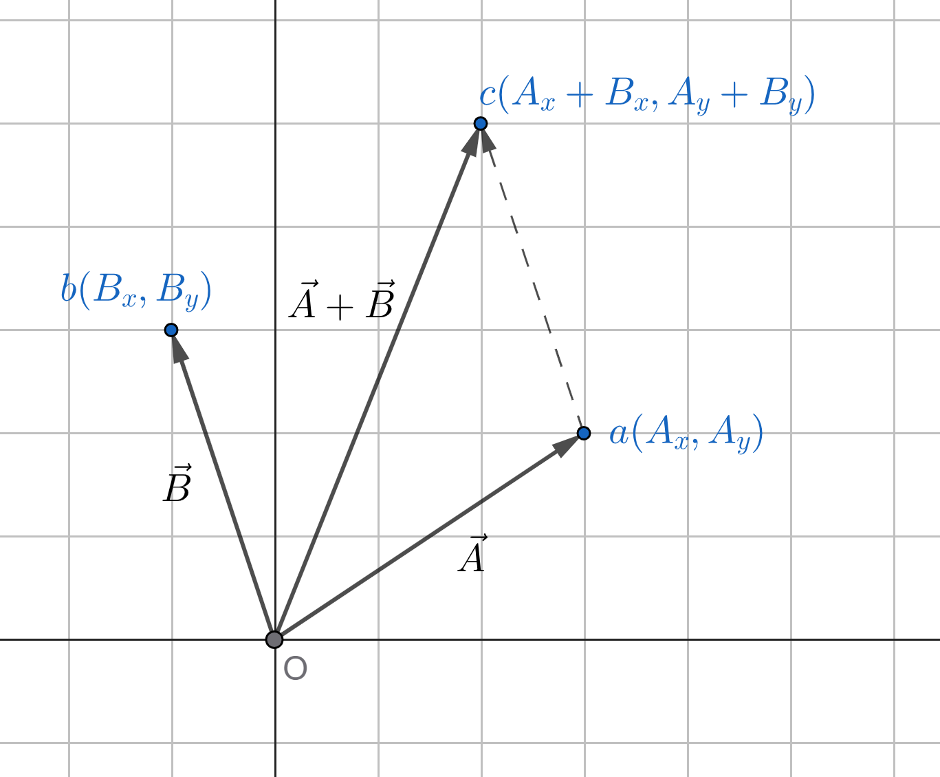
Clearly, the two vectors can be added using the Triangle law i.e. by putting the tail of \(\vec{B}\) on the head of \(\vec{A}\) (represented using dotted vector in the figure), and then tracing the resultant vector, \((\vec{A} + \vec{B})\) from the tail of \(\vec{A}\) to the head of \(\vec{B}\) as is done.

What we see here is that: the vector \(\vec{B}\) "drags" the head of vector \(\vec{A}\) the same amount as its components and vice versa. For reference, the grid lines has been shown. Hence, the resultant vector \((\vec{R})\) can be written in the coordinate form as: $$ \begin{align} \vec{R} &= \vec{A} + \vec{B} \\[4px] \vec{R} &= (A_x\,\hat{i} + A_y\,\hat{j}) + (B_x\,\hat{i} + B_y\,\hat{j}) \\[4px] \vec{R} &= (A_x + B_x)\, \hat{i} + (A_y + B_y)\, \hat{j} \qquad \color{red}{(3.4)} \end{align} $$

The economy here is really appreciable. In the abstract form of addition of vectors, first we would have to find the magnitude of the resultant vector using \(\text{eq} (2.1)\) and then determine its direction with respect to initial vectors using \(\text{eq} (2.2)\). Finally, we draw the resultant vector. But, in the component form, we just need to do the algebraic addition for the components and, lo and behold, we got the resultant vector.

Anyway, it should be emphasized that both the forms of addition are important and we are not showing one above the another. It is just the situation under which we are performing addition, which makes this apparent scenario of better form of addition.



• In 3 dimensions:

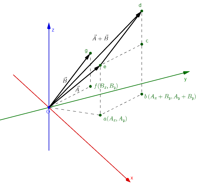
Having done in the two dimensions, it is almost trivial to generalize it to three dimensions. Again, consider two vectors \(\vec{A}\) and \(\vec{B}\) given as:



$$ \begin{align} \vec{A} = A_x \, \hat{i} + A_y \, \hat{j} + A_z \, \hat{k} \\[4px] \vec{B} = B_x \, \hat{i} + B_y \, \hat{j} + B_z \, \hat{k} \\[4px] \end{align} $$

These are shown in the Figure 3.4. It might take a little time to digest all the information in the diagram. To interactively explore (change the camera angle) this diagram, visit this Geogebra resource link.

A similar thing as above has happened here too. The vector \(\vec{B}\) "drags" the vector \(\vec{A}\) towards itself by the same amount as its coordinates. The \(2D\) drag can be explicity seen on the \(xy\)-plane: the projection of vector \(\vec{A}\) on the plane i.e. \(a(A_x, A_y)\) is dragged by the projection of \(\vec{B}\) i.e. \(f(B_x, B_y)\) to make it \(b(A_x + B_x, A_y + B_y)\), which is the projection of the final vector \(\vec{A} + \vec{B}\). All of this is backed by the Triangle Law (see the \(\triangle oed\) in figure, which utilizes the triangle law of vector addition to add the two vectors).

The crutial distinction comes here by the addition of the third components (the \(z\)-components). The \(z\)-component of \(\vec{A}\) was at point \(e(A_x, A_y, A_z)\) which get "dragged" to the point \(d(A_x + B_x, A_y + B_y, A_z + B_z)\), by the vector \(\vec{B}\text{'s}\) \(z\)-component, which lies at \(g(B_x, B_y, B_z)\). Which is to say: \(cd = fg\). One last thing worth mentioning is that: all the things discussed here can be done equally well in terms of \(\vec{A}\) dragging the components of \(\vec{B}\).

So, now we are ready to write the sum of the two vectors as: $$ \begin{align} \vec{R} &= \vec{A} + \vec{B} \\[4px] \vec{R} &= (A_x \, \hat{i} + A_y \, \hat{j} + A_z \, \hat{k}) + (B_x \, \hat{i} + B_y \, \hat{j} + B_z \, \hat{k}) \\[4px] \vec{R} &= (A_x + B_x) \, \hat{i} + (A_y + B_y) \, \hat{j} + (A_z + B_z) \, \hat{k} \qquad \color{red}{(3.5)} \end{align} $$

• Negation of vector in component form:

The negation of a vector in component form follows simply in this scenario. Consider again the vector: $$ \vec{A} = A_x \, \hat{i} + A_y \, \hat{j} + A_z \, \hat{k}. $$

Let \(\vec{A^n}\) (here, \(n\) is just a ^superscript to represent 'negative' and should not be considered as an exponent) be the vector equal and opposite to \(\vec{A}\), then using vector sum, we get: $$ \begin{align} &\vec{A} + \vec{A^n} = \vec{0} \\[4px] \implies & \begin{aligned} (A_x + A_x^n)\, &\hat{i} + (A_y + A_y^n)\, \hat{j} + (A_z + A_z^n)\, \hat{k} \\ &= 0 \, \hat{i} + 0 \, \hat{j} + 0 \, \hat{k} \end{aligned}\\[4px] \implies &\begin{cases} A_x + A_x^n = 0 \\[4px] A_y + A_y^n = 0 \\[4px] A_z + A_z^n = 0 \\[4px] \end{cases} \implies \begin{cases} A_x^n = -A_x \\[4px] A_y^n = -A_y \\[4px] A_z^n = -A_z \\[4px] \end{cases} \end{align} $$

So, the negation of \(\vec{A}\) would be given as: $$ \begin{align} \vec{A^n} &= -\vec{A} = (-A_x) \, \hat{i} + (- A_y) \, \hat{j} + (- A_z) \, \hat{k} \\[4px] \implies -\vec{A} &= -A_x \, \hat{i} - A_y \, \hat{j} - A_z \, \hat{k} \qquad \color{red}{(3.6)} \end{align} $$



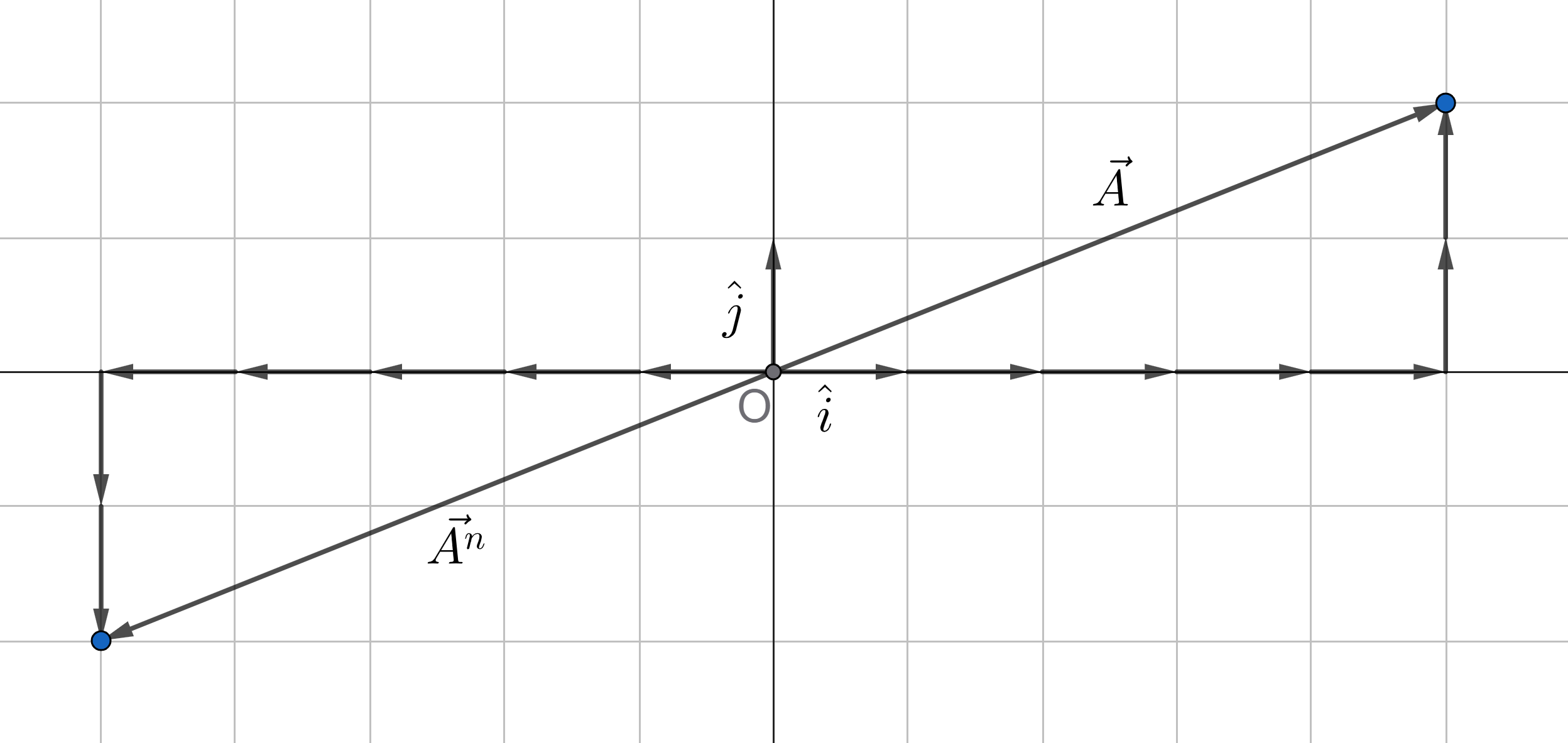
i.e. all the components of the vector is negated to get the required equal and opposite vector. This can easily be justified using diagrams similar to figure 3.5.

• Null vector:

If you noticed, we used the vector arrow on zero above in the analysis, as \(\vec{0}\). This is known as the 'Null Vector'. It was intoduced above in the case of vector addition when we needed the resultant to be zero \((\vec{A} + \vec{A^n} = \vec{0})\). Since, vector addition gives resultant as a vector, we need to put an arrow over zero to show that it is a vector with magnitude zero.

Now, to interpret it we say that the Null vector is a vector with magnitude zero and can point in any direction we wish. So, it has no magnitude (in the sense of arrow length), and no specific direction. Since, the magnitude is zero, we can easily see that: $$ \vec{0} = 0 \,\hat{i} + 0 \,\hat{j} + 0 \,\hat{k} \qquad \color{red}{(3.7)} $$