Mathematical Methods
The reader is assumed to have some basic understanding of geometry and algebra.
Topics covered in this section are as follows:
* Further topics would be added based on need.
1. Basic Geometry
- Pythagoras Theorem:
- Proof:
- Distance Formula for 2 and 3 dimensions:
- 2 dimensional case:
- 3 dimensional case:
triangle
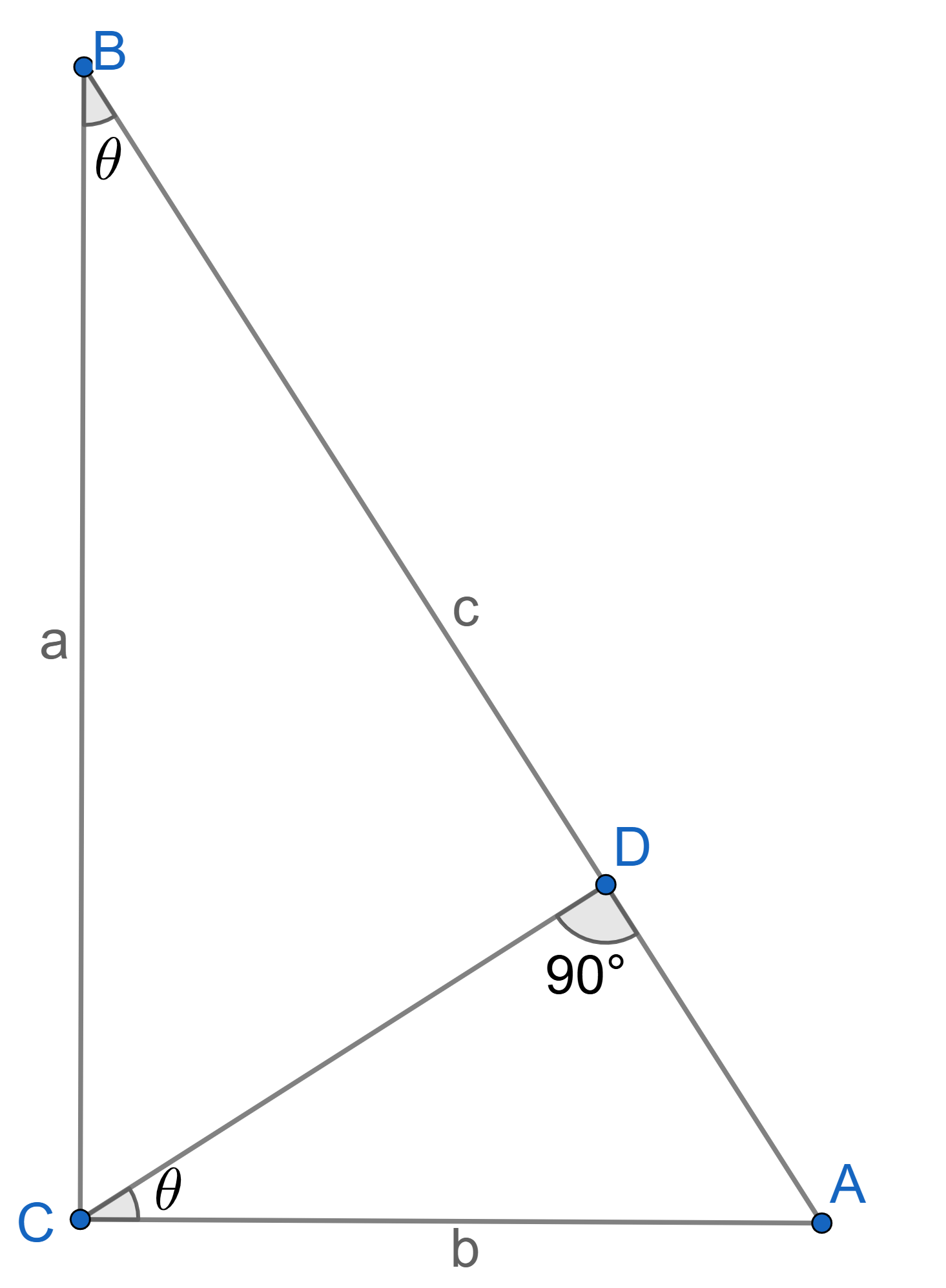
For a right angled triangle, as shown in Figure 1.1, with the hypotenuse \(c\), base \(b\), and height \(a\):
$$c^2=a^2+b^2 \hspace{1cm} \color{red}{(1.1)}$$
This relation was given by ancient Greek philosopher, Pythagoras upon whom the theorem is named.
This thorem would be used for finding most prominantly the length of vectors, followed by its traditional applications in finding the side length of right-angled triangles and much more.
Here is a simple proof using triangle similarity.
Consider the Figure 1.1 again for \(\triangle BCD\) and \(\triangle ABC\). Clearly,
$$
\begin{align}
\angle CBD &= \angle CBA =\theta \\
\angle BCD &= \angle BAC =90^{\circ}-\theta \\
\angle BDC &= \angle BCA =90^{\circ}
\end{align}
$$
This shows that the \(\triangle BCD \sim \triangle ABC, \) by the \(AAA\) similarity criterion. A similar argument for \(\triangle ACD\) and \(\triangle ABC\) would give \(\triangle ACD \sim \triangle ABC. \)
Using similarity,
$$\frac{BC}{BD}=\frac{AB}{BC}\implies BD= \frac{BC^2}{AB}\hspace{1cm}(\text{i})$$
and
$$\frac{AB}{AC}=\frac{AC}{AD}\implies AD= \frac{AC^2}{AB}\hspace{1cm}(\text{ii})$$
Using,\((\)i\()\) and \((\)ii\()\) and using the fact that \(AD+BD=AB\), we get:
The distance formula is used to calculate the distance between two points in space. Now, the space can be of any dimensions (at least, theoretically) but, for now, we are concerned with only the 2 and 3 dimensional space.
Lets consider them both one by one.
For two points in the two dimensional plane, say \(A(x_1,y_1)\) and \(B(x_2,y_2)\), the distance between them is: $$r=\sqrt{(x_2-x_1)^2+(y_2-y_1)^2} \hspace{1cm} \color{red}{(1.2)}$$
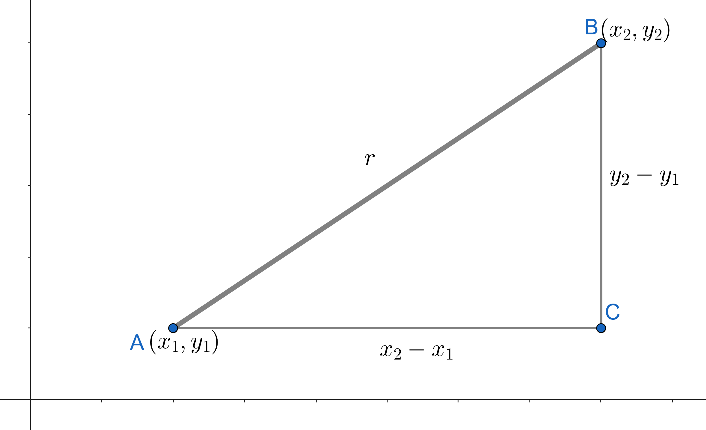
Consider the Figure 1.2 shown. The points \(A\) and \(B\) are shown, with the horizontal distance along the \(x\)-axis as \(x_2-x_1\) and the vertical distance along the \(y\)-axis as \(y_2-y_1\). Further, we apply the Pythagoras Theorem to the \(\triangle ABC\), so as to find the length of side \(AB\) using the sides \(AC\) and \(BC\), as below.
This shows the equation \(1.2\).
In the three dimensional "normal" space, the distance between two points \(A(x_1,y_1,z_1)\) and \(B(x_2,y_2,z_2)\) is given by: $$r=\sqrt{(x_2-x_1)^2+(y_2-y_1)^2+(z_2-z_1)^2} \hspace{1cm} \color{red}{(1.3)}$$
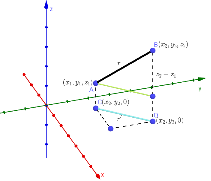
Now, to start with we first project the points \(A\) and \(B\) to the \(x-y\) plane turning them into \(C(x_1,y_1,0)\) and \(D(x_2,y_2,0)\), respectively as shown. Further, we apply the 2 dimensional distance formula (Eq 1.2) for finding the distance \(r'\) to be: $$r'= \sqrt{(x_2-x_1)^2+(y_2-y_1)^2}$$ The above equation is easily verified by comparing the top view (Figure 1.4) shown below with the Figure 1.2. We identify that the length of the green and the blue segments are the same i.e. \(r'\). And, the vertical distance of the point \(A\) and \(B\) or the green segment and the point \(B\) is \(\left(z_2-z_1\right)\).
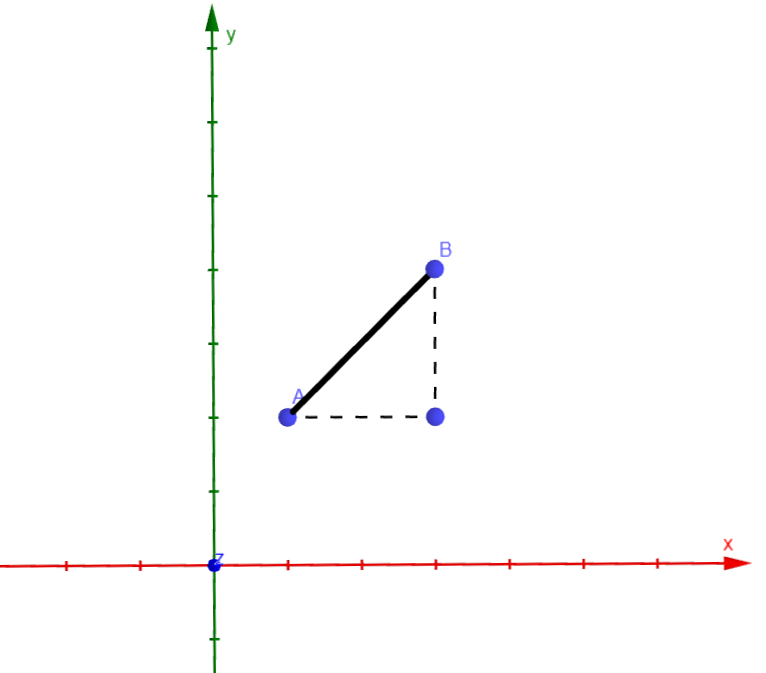
Then, we again employ the Pythagoras theorem, this time for the triangle with two vertices as \(A\) and \(B\) and the green segment as the base. So, we get: $$ \begin{aligned} r &= \sqrt{(r')^2+(z_2-z_1)^2} \\ \implies r&= \sqrt{(x_2-x_1)^2+(y_2-y_1)^2+(z_2-z_1)^2} \end{aligned} $$ By this, we have proved the distance formula in 3-dimensions.
One special case: A case which arises very frequently, especially when dealing with vectors, is the distance of a point, say \((x,y,z)\) from the origin \((0,0,0)\). Using equation 1.3 ,we get this distance to be: $$ r = \sqrt{x^2+y^2+z^2} \hspace{2cm} \color{red}{(1.4)} $$ This is often referred as the length of a vector from origin to the point \((x,y,z)\).
2. Trigonometry
Trigongometry is the study of angles, more specifically the study of angles of a triangle. We start by defining some some relations in between the angle and side length of the right angled triangle, and move towards a general form.
- Some definitions:
-
Sine of \(\theta\) :
Sine of angle \(\theta\) is defined as the ratio of the length of the perpendicular and the hypotenuse and is denoted as: $$ \sin{\theta}=\frac{p}{h} \hspace{1cm} \color{red}{(2.1)} $$
Upon rearranging, we get \(p=h \sin{\theta}\). Thus, \(p\) is said to be the projection of \(h\) over the perpendicular side. This is much useful when dealing with vector projection. Further, we see from \(\angle CAB\) that: $$ \begin{align} \sin{(90^{\circ}-\theta)} &= \frac{b}{h} = \cos{\theta} \\[4px] \implies \sin{(90^{\circ}-\theta)} &= \cos{\theta} \hspace{1cm} \color{red}{(2.1 \text{ i})} \end{align} $$ This is done using the definition of \(\cos{\theta}\) (see below).
-
Cosine of \(\theta\) :
Cosine of angle \(\theta\) is defined as the ratio of the length of the base and the hypotenuse and is denoted as: $$ \cos{\theta}=\frac{b}{h}\hspace{1cm} \color{red}{(2.2)} $$
As before, \(b=h \cos{\theta}\). Thus, \(b\) is the projection of \(h\) on the base. Again, $$\cos{(90^{\circ}-\theta)}= \sin{\theta} \hspace{1cm} \color{red}{(2.2 \text{ i})}$$ This relation's extension to all the trigonometric functions is left to the reader as an exercise.
-
Tangent of \(\theta\) :
Tangent of angle \(\theta\) is the ratio of sine and cosine of \(\theta\) or, length of the perpendicular and the base. It is denoted as: $$ \tan{\theta}=\frac{\sin{\theta}}{\cos{\theta}}=\frac{p}{b} \hspace{1cm}\color{red}{(2.3)} $$ Now, \(\tan{\theta}\) has an immense significance as it represents the slope (how slant is the line with respect to the \(x\)-axis) of the hypotenuse.
-
Cosecant of \(\theta\) :
It is defined as the reciprocal of sine. It is denoted as \(\csc{\theta}\) or sometimes \(\text{cosec }\theta\) i.e. $$ \csc{\theta}=\frac{1}{\sin{\theta}}=\frac{h}{p} $$
-
Secant of \(\theta\) :
It is defined as the reciprocal of cosine. It is denoted as \(\sec{\theta}\) i.e. $$ \sec{\theta}=\frac{1}{\cos{\theta}}=\frac{h}{b} $$
-
Cotangent of \(\theta\) :
It is defined as the reciprocal of tangent. It is denoted as \(\cot{\theta}\) i.e. $$ \cot{\theta}=\frac{1}{\tan{\theta}}=\frac{b}{p} $$
- Pythagorean Trigonometric Identities:
- Fundamental Pythagorean Identity:
- Other pythagorean identities:
- Review and talk on angles:
- Relation between degree and radian:
- An important relation:
- Redefining trigonometric functions:
- Function of negative acute angles:
- Function of any real angle:
- Angle Sum relations:
- For sine :
- For cosine:
- For tangent:
- For other trigonometric functions:
- Some important results:
With all the theoretical framework in our hand, let's calculate some trigonometric identities which would prove to be helpful in our ananlysis later on.
- \(\underline{\sin{(2\theta)}}\)
- \(\underline{\cos{(2\theta)}}\)
- \(\underline{\sin{(3\theta)}}\)
Using, \(\text{eq(2.17 i)}\) for \(\theta = \phi\), we get: $$ \begin{align} \sin{(2\theta)} &= \sin{(\theta + \theta)} \\[4px] \implies \sin{(2\theta)} &= \sin{\theta}\cos{\theta} + \cos{\theta}\sin{\theta} \\[4px] \implies \sin{(2\theta)} &= 2\sin{\theta}\cos{\theta} \hspace{1cm} \color{red}{\text{(2.21)}} \\ \end{align} $$ This equation is much important when simplifying trigononmetric equations in our analysis.
Using, \(\text{eq(2.18 i)}\) for \(\theta = \phi\), we get: $$ \begin{align} \cos{(2\theta)} &= \cos{(\theta + \theta)} \\[4px] \implies \cos{(2\theta)} &= \cos{\theta}\cos{\theta} - \sin{\theta}\sin{\theta} \\[4px] \implies \cos{(2\theta)} &= \cos^2{\theta} - \sin^2{\theta} \hspace{1cm} \color{red}{\text{(2.22)}} \\[4px] &= 2\cos^2{\theta} - 1 \\[4px] &= 1 -2\sin^2{\theta} \\ \end{align} $$ The last two steps of conversion uses the relation \(\text{eq (2.4)}\) i.e. \(\sin^2{\theta}+ \cos^2{\theta} = 1\). Again, the three forms are equivalent in terms of mathematics and also in terms of use in the analysis. In a similar way, we can deduce higher order \(\sin\) and \(\cos\) i.e. for \(3\theta\) or maybe \(4\theta\). But, we would rarely need them. One is done here:
Again, using \(\text{eq(2.17 i)}\) for \(\theta = \phi\), we get: $$ \begin{align} \sin{(3\theta)} &= \sin{(2\theta + \theta)} \\[4px] \implies \sin{(3\theta)} &= \sin{(2\theta)}\cos{\theta} + \cos{(2\theta)}\sin{\theta} \\[4px] \implies \sin{(3\theta)} &= 2\sin{\theta}\cos{\theta}\cos{\theta} + (\cos^2{\theta}-\sin^2{\theta})\sin{\theta} \\[4px] \implies \sin{(3\theta)} &= 2\sin{\theta}\cos^2{\theta} + \cos^2{\theta}\sin{\theta}-\sin^3{\theta} \\[4px] \implies \sin{(3\theta)} &= 3\sin{\theta}(1-\sin^2{\theta}) -\sin^3{\theta} \\[4px] \implies \sin{(3\theta)} &= 3\sin{\theta} -4\sin^3{\theta} \hspace{1cm} \color{red}{\text{(2.23)}} \\[4px] \end{align} $$
Here, we used the last two results along with the angle sum relation. For, cosine it turns out to be (left as an exercise): $$ \cos{(3\theta)} = 4\cos^3{\theta} - 3\cos{\theta} \hspace{1cm} \color{red}{(2.24)} $$
Consider the figure shown.
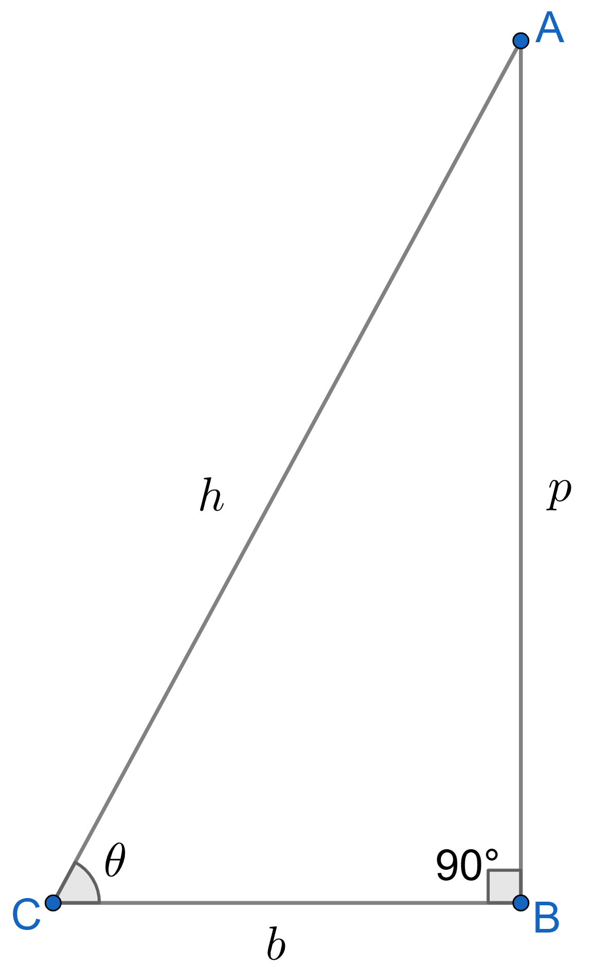
with side lengths
The three sides of the triangle \(ABC\), base \(BC\) has length \(b\), perpendicluar (the side in front of the angle under consideration, here, \(\theta\)) \(AB\) has length \(p\) and the longest side, hypotenuse (the side in front of right angle) \(AC\) has length \(h\).
We define the following:
| Function ↓ \( \theta\) | \(0^{\circ}\) | \(30^{\circ}\) | \(45^{\circ}\) | \(60^{\circ}\) | \(90^{\circ}\) |
|---|---|---|---|---|---|
| \(\sin{\theta}\) | \(0\) | \(1/2\) | \(1/\sqrt{2}\) | \(\sqrt{3}/2\) | \(1\) |
| \(\cos{\theta}\) | \(1\) | \(\sqrt{3}/2\) | \(1/\sqrt{2}\) | \(1/2\) | \(0\) |
| \(\tan{\theta}\) | \(0\) | \(1/\sqrt{3}\) | \(1\) | \(\sqrt{3}\) | \(\inf \)* |
| \(\csc{\theta}\) | \(\inf \)* | \(2\) | \(\sqrt{2}\) | \(2/\sqrt{3}\) | \(1\) |
| \(\sec{\theta}\) | \(1\) | \(2/\sqrt{3}\) | \(\sqrt{2}\) | \(2\) | \(\inf \)* |
| \(\cot{\theta}\) | \(\inf \)* | \(\sqrt{3}\) | \(1\) | \(1/\sqrt{3}\) | \(0\) |
| *here, \(\inf\) represents infinity or undefined | |||||
Some of the real "building block" identities of trigonometry are as follows:
To start with, consider the Figure 2.1 again. Let's try to calculate the sum of square of \(\sin{\theta}\) and \(\cos{\theta}\): $$ \begin{align} \sin^2{\theta} + \cos^2{\theta} &= \left(\frac{p}{h}\right)^2 + \left(\frac{b}{h}\right)^2 \\ \implies \sin^2{\theta} + \cos^2{\theta} &= \frac{p^2 + b^2}{h^2}\\ \implies \sin^2{\theta} + \cos^2{\theta} &= \frac{h^2}{h^2} \\ \implies \sin^2{\theta} + \cos^2{\theta} &= 1 \hspace{1cm} \color{red}{(2.4)} \end{align} $$ The last equation (Eq. 2.4) is the required fundamental pythagorean identity. We have used the pythagoras theorem to proceed to the third equation from second.
Two other pythagorean identities are:
$$ \begin{align} 1 + \tan^2{\theta} &= \sec^2{\theta} \hspace{1cm} \color{red}{(2.5)} \\[5pt] 1 + \cot^2{\theta} &= \csc^2{\theta} \hspace{1cm} \color{red}{(2.6)} \end{align} $$
These are easily derived from the fundamental identity, as equation 2.5 can be derived by dividing the equation 2.4 on both sides by \(\cos^2{\theta}\) and equation 2.6, by dividing both side of 2.4 by \(\sin^2{\theta}\), as is done below: $$ \begin{align} &\sin^2{\theta} + \cos^2{\theta} = 1 \\[4pt] \implies &\frac{\sin^2{\theta} + \cos^2{\theta}}{\cos^2{\theta}} = \frac{1}{\cos^2{\theta}} \\[4pt] \implies &\tan^2{\theta} + 1 = \sec^2{\theta} \end{align} $$ and $$ \begin{align} &\sin^2{\theta} + \cos^2{\theta} = 1 \\[4pt] \implies &\frac{\sin^2{\theta} + \cos^2{\theta}}{\sin^2{\theta}} = \frac{1}{\sin^2{\theta}} \\[4pt] \implies &1 + \cot^2{\theta} = \csc^2{\theta} \end{align} $$ These identities are extremely useful for analyzing trigonometry further, as we would see in the upcoming sections.Till now, we have been handling angles in degrees as one can see in table 2.1. By convention, \(360^{\circ}\) is the whole angle about a point. Further, we say that the right angle is \(90^{\circ}\) and so on. Now, we move towards defining a new unit of angle measure, raidans.
One radian is defined as the angle subtended at the center of circle by an arc of length equal to the radius, of the circle in consideration. This is shown in the figure 2.2.
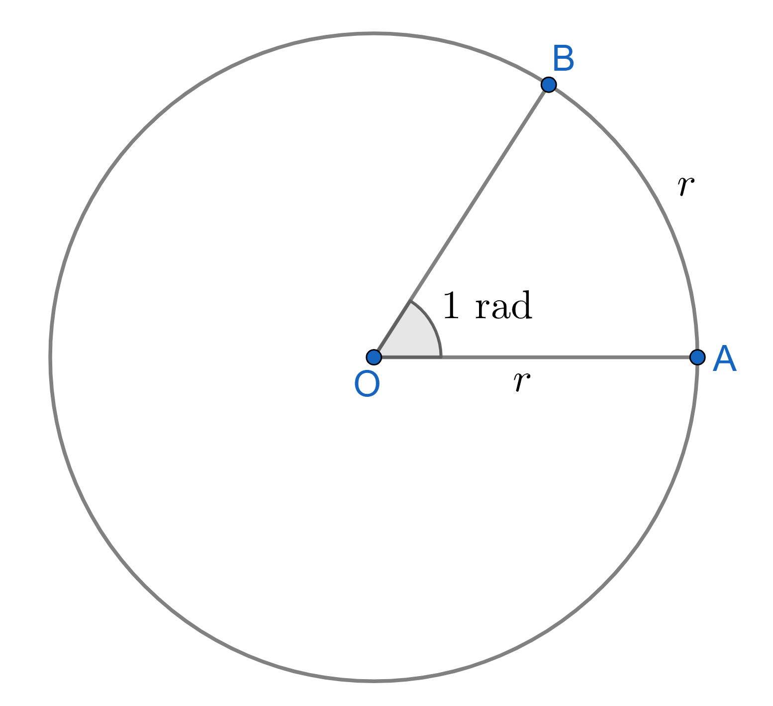
It is often denoted simply as "rad" or sometimes by superscripting the angle value by "c" (example, \(1^{\text{c}}\)). Also, if no any unit has been mentioned, then the unit is considered to be radians.
But why is the shift from degrees to radians is required? The answer is quite simple: because radian is a natural measure of angle, while degree is just an arbitrary convention. Radian pops up in differentiation, Taylor's theorem, and even in simple geometry, as we will observe in due course.
Consider the figure 2.2 again. The total angle about the point O is \(360^{\circ}\) in degrees. Also, one radian is the angle subtended by the arc of length \(r\), at the center. Further, since the circumference of circle with radius \(r\) is \(2\pi r\), so there can be $$ \frac{2\pi r}{r} = 2\pi $$ arcs of length \(r\) about the whole circumference. This gives the total angle to be \(2\pi\) rads about the point O in the circle.
The above argument shows that: $$ \begin{align} 360^{\circ} &= 2\pi \text{ rads} \hspace{2cm} \color{red}{(2.7)}\\[4px] \implies 1^{\circ} &= \frac{2\pi}{360} \text{ rads} \implies \boxed{1^{\circ}= \frac{\pi}{180} \text{ rads}} \end{align} $$ and $$ \boxed{1\text{ rad}= \left(\frac{180}{\pi}\right)^{\circ}} $$ One can check the following easily:
| Degree\(^{\circ}\) | Radian\(^{\text{c}}\) |
|---|---|
| \(0\) | \(0\) |
| \(30\) | \(\pi/6\) |
| \(45\) | \(\pi/4\) |
| \(60\) | \(\pi/3\) |
| \(90\) | \(\pi/2\) |
| \(120\) | \(2\pi/3\) |
| \(180\) | \(\pi\) |
| \(...\) and so on. | |
By now, it should be clear that there is some relation between the radius, arc length and angle and angle subtended at the center of the circle. This relation looks really neat when the angle is taken in unit of radian. Let's now turn to it.
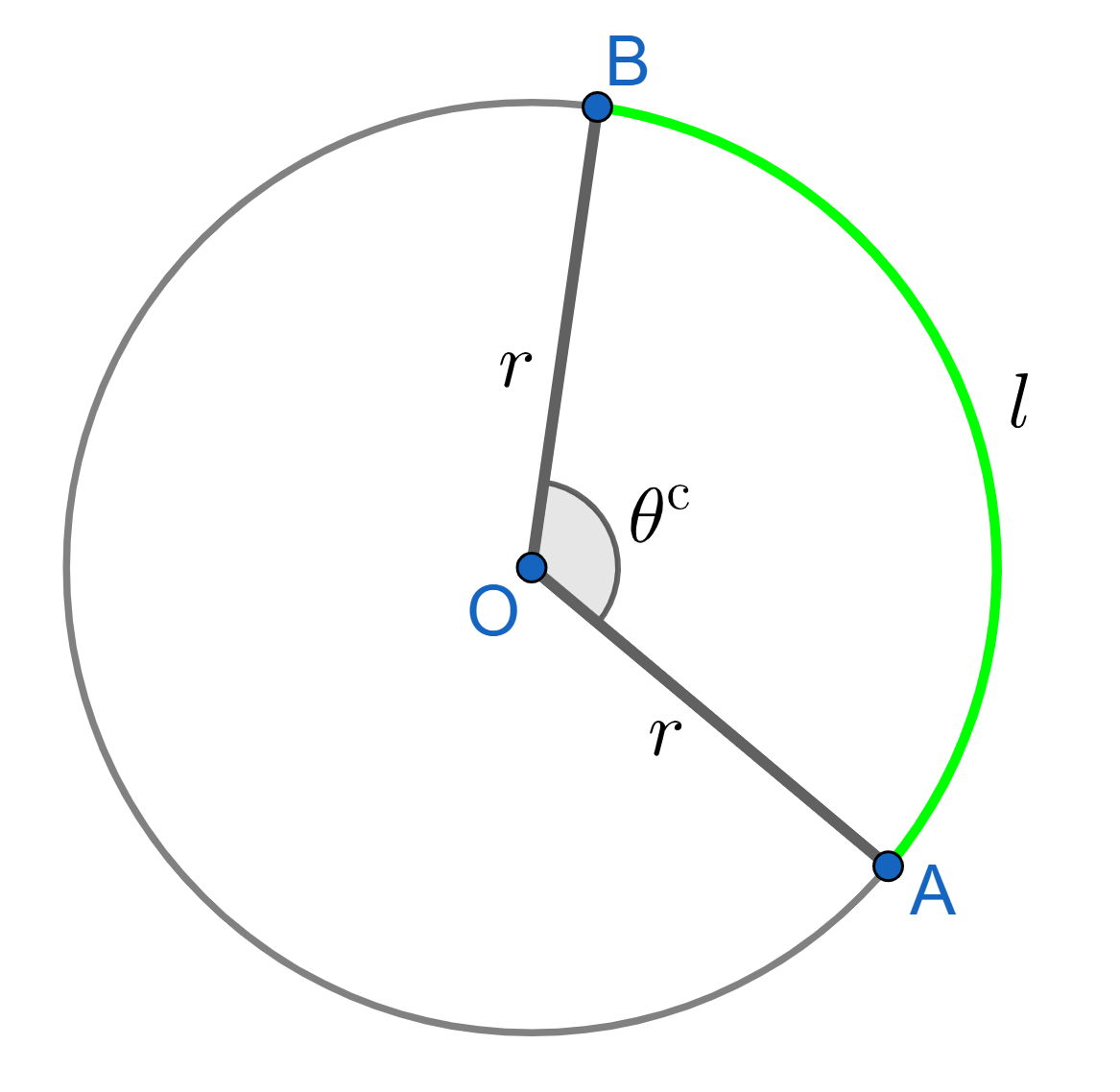
of length \(l\) in radians
Say, we have a circle with radius \(r\) and consider an arc of length \(l\) about the cicumference that subtends an angle \(\theta \text{ rads}\) at the center if the circle, as in figure 2.3. Clearly, number of arcs (in the mathematical sense) of length \(r\) contained in length \(l\) is \(l/r\). And since, each such arc subtends one radian at the center of the circle, total angle subtended by the arc of length \(l\) is: $$ \theta^{\text{ c}} = \frac{l}{r} \hspace{1cm} \color{red}{(2.8)} $$ The superscript \(^\text{c}\) over \(\theta\) indicates that the angle should be measured in radians for this relation to hold.
Clearly, this relation can be restated by measuring the angle in degrees using eq 2.7 in eq 2.8 to get: $$ \theta^{\circ} = \frac{\pi}{180}\left(\frac{l}{r}\right) $$ Here, the superscript \(^\circ\) over \(\theta\) indicates the angle is to be measured in degrees. One can see that the relation in radians is more intuitive and natural than that in degrees.
The definition of trigonometric functions, as in the first section, was totally based on lengths and was valid only for acute angles, which makes the functions to be positive only. And this is enough to work in analytical geometry. But, to understand our surrounding better, we needed the sine and cosine for all real numbers, as we would see soon. To facilitate this, we need to redefine those functions.
The redifinition is done such that we can encompass all the real numbers as its domain (the input we provide to a function). For this, we use a unit circle (circle with radius 1), as shown in figure 2.4.
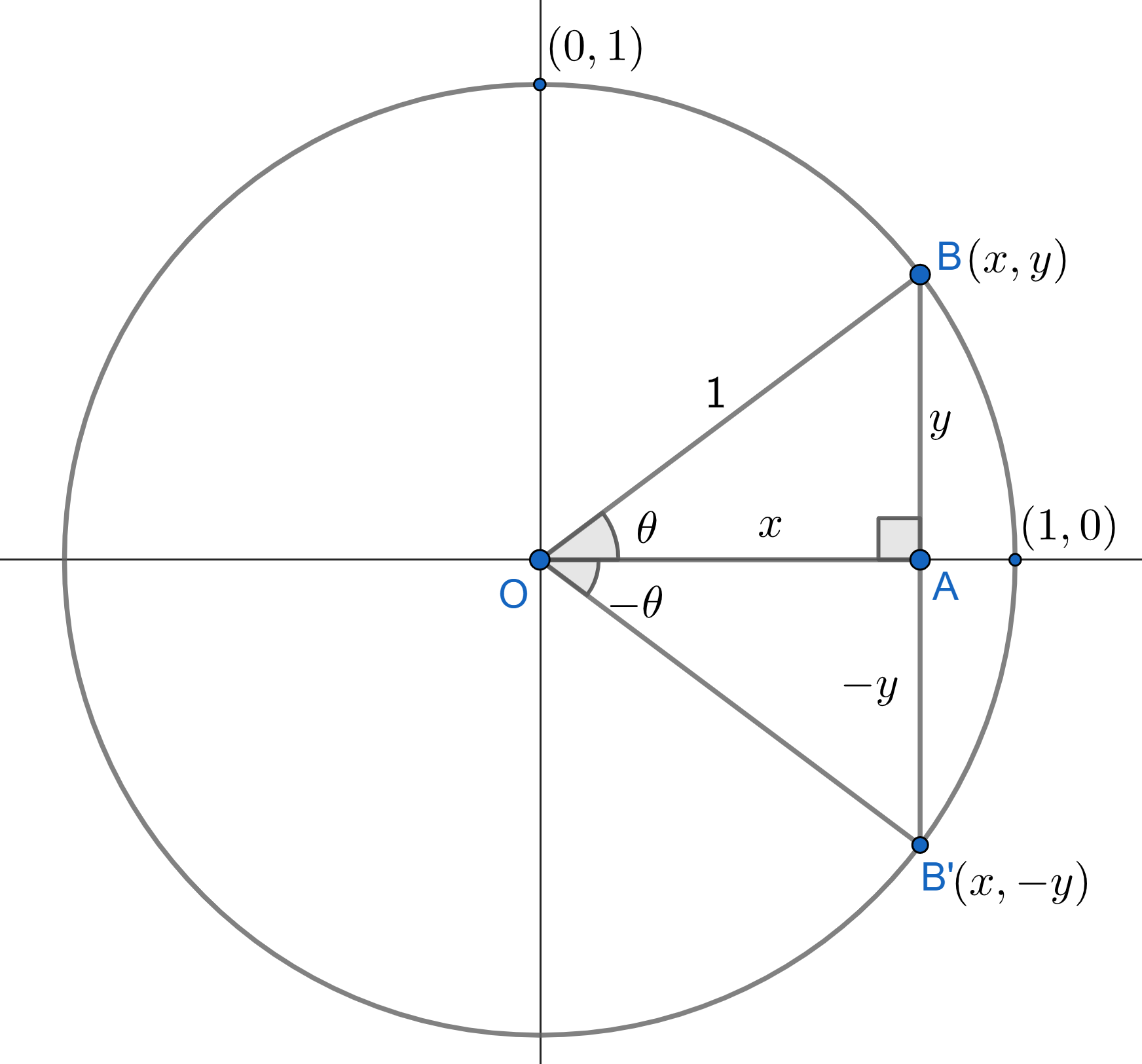
From the previous definition,
$$ \begin{align} \cos{\theta} &= \frac{OA}{OB} = x \hspace{1cm} \color{red}{(2.9\text{ i})}\\[4px] \sin{\theta} &= \frac{AB}{OB} = y \hspace{1cm} \color{red}{(2.9\text{ ii})} \end{align} $$
If we consider this to be the base definition of sine and cosine with \(x\) and \(y\) as the coordinates (including sign) of the point making angle \(\theta\) with \(x\)-axis through the origin O as the vertex, then we can easily extend out these functions to all real numbers. To say,
Sine of an angle \(\theta\), the angle subtended by a line segment (for refrence, OB in figure), with the \(x\)-axis at the center of a unit circle on which B is lying, is given as the ratio of \(y\)-coordinate (with sign) of point B and the length (always positive) of the hypotenuse (or line segment OB) i.e.
$$ \sin{\theta} = \frac{y}{|OB|} = y $$ Similarly, $$ \cos{\theta} = \frac{x}{|OB|} =x $$This can be extended to other trigonometric functions in a similar way.(from here, we refer to all trigonometric functions just by saying "functions" in this section).
We begin by extending our analysis to the negative real numbers first, before moving beyond the acute angles. Again consider the figure 2.4. We have, \(\sin{\theta} = y\). And, using our new definition (from figure): $$ \begin{align} \sin{(-\theta)} &= \frac{-y}{|OB'|} = -y \\[4px] \implies \sin{(-\theta)} &= - \sin{\theta} \hspace{1cm} \color{red}{(2.10 \text{ i})} \end{align} $$ Further, \(\cos{\theta} = x\) and from figure,
$$ \begin{align} \cos{(-\theta)} &= \frac{x}{|OB'|} = x \\[4px] \implies \cos{(-\theta)} &= \cos{\theta} \hspace{1cm} \color{red}{(2.10 \text{ ii})} \end{align} $$
For \(\tan{(-\theta)}\), we have: $$ \begin{align} \tan{(-\theta)} &= \frac{\sin{(-\theta)}}{\cos{(-\theta)}} \\[4px] \implies \tan{(-\theta)} &= \frac{-\sin{\theta}}{\cos{\theta}} = -\tan{\theta} \hspace{1cm} \color{red}{(2.10 \text{ iii})} \end{align} $$ A similar extension to other trigonometric functions can be done, leading to : $$ \begin{align} \csc{(-\theta)} &= -\csc{\theta} \\ \sec{(-\theta)} &= \sec{\theta} \\ \cot{(-\theta)} &= -\cot{\theta} \end{align} $$
By the title, "function of any real angle" we mean that, having done with the function of negative acute angle, we now move to expanding this system to any real number in terms of the known value of acute angles.
corresponding angle \(\theta\)
For angles between \(\pi/2\) and \(\pi\):
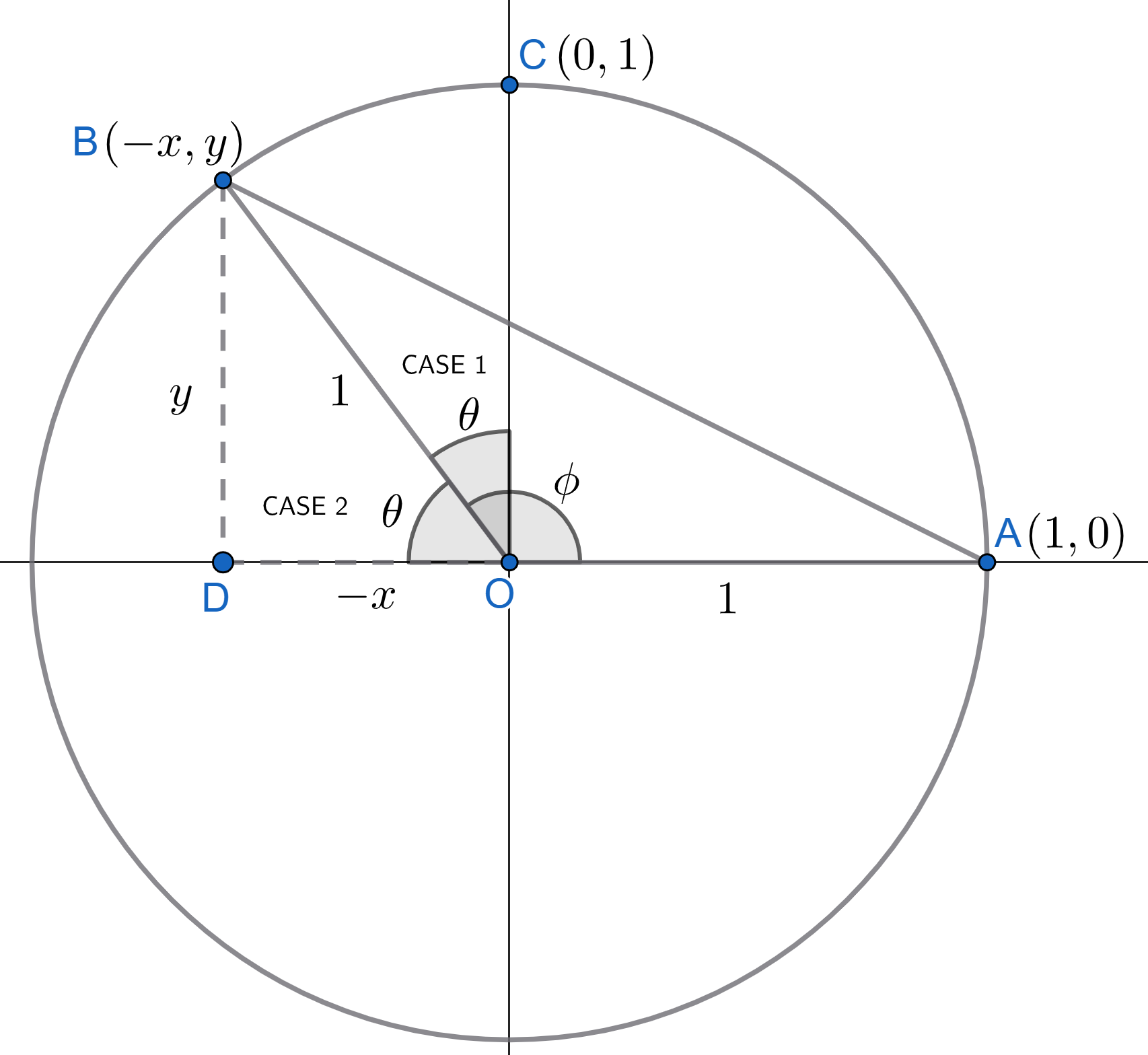
Consider an angle \(\phi\) \((\pi/2 \le \phi \leq \pi )\) as shown in figure 2.5. We want to find \(\sin{\phi}\). This can be written as:
CASE 1: \((\pi/2 + \theta = \phi)\)
$$
\begin{align}
\sin{\phi} &= \sin{\left(\frac{\pi}{2} + \theta\right)} \\[4px]
&= \sin{\left(\frac{\pi}{2}- (-\theta)\right)}\\[4px]
&= \cos{(-\theta)}\hspace{1cm} \text{(using eq (2.1 i))}\\[6px]
\sin{\left(\frac{\pi}{2}+\theta\right)} &= \cos{\theta} \hspace{1cm} (\text{using eq (2.11)}) \hspace{1cm} \color{red}{(2.11 \text{ i})}
\end{align}
$$
This relation is useful for finding sine of angles greater than \(90^{\circ}\), here \(\phi\), till the angle \(\theta\) is acute, as we know geometrically,the values of trigonometric functions for acute angles only. This is done for cosine as below:
$$ \begin{align} \cos{\phi} &= \cos{\left(\frac{\pi}{2} + \theta\right)} \\[4px] &= \cos{\left(\frac{\pi}{2}- (-\theta)\right)}\\[4px] &= \sin{(-\theta)}\hspace{1cm} \text{(using eq (2.2 i))}\\[6px] \cos{\left(\frac{\pi}{2}+\theta\right)} &= -\sin{\theta} \hspace{1cm} (\text{using eq (2.10)}) \hspace{1cm} \color{red}{(2.11 \text{ ii})} \end{align} $$
Using, these we can find this relation for tan function : $$ \begin{align} \tan{\left(\frac{\pi}{2}+\theta\right)} &= \frac{\sin(\frac{\pi}{2}+\theta)}{\cos{(\frac{\pi}{2}+\theta)}}\\[4px] &=\frac{\cos{\theta}}{-\sin{\theta}}\\[4px] \tan{\left(\frac{\pi}{2}+\theta\right)} &= -\cot{\theta} \hspace{1cm} \color{red}{(2.11 \text{ iii})} \end{align} $$ This can be extended to other trigonometric functions in a similar way, to find the following: \begin{align} \csc{\left(\frac{\pi}{2}+\theta\right)} &= \sec{\theta} \\[4px] \sec{\left(\frac{\pi}{2}+\theta\right)} &= -\csc{\theta}\\[4px] \cot{\left(\frac{\pi}{2}+\theta\right)} &= -\tan{\theta} \end{align}
CASE 2: \((\phi + \theta = \pi)\) Here, \(\sin{\phi}\) can be written as: (from figure 2.5) $$ \begin{align} \sin{\phi} &= \sin{(\pi-\theta)} \\[4px] &= \sin{\left(\frac{\pi}{2}-\left(\theta - \frac{\pi}{2}\right)\right)}\\[4px] &= \cos{\left(\theta - \frac{\pi}{2}\right)} \hspace{1.5cm} (\text{using eq (2.1 i)} ) \\[6px] \sin{(\pi-\theta)} &= \cos{\left(-\left(\frac{\pi}{2} - \theta\right)\right)} \\[4px] &= \cos{\left(\frac{\pi}{2}-\theta\right)} \hspace{1.5cm} (\text{using eq (2.11)}) \\[6px] \sin{(\pi-\theta)} &= \sin{\theta} \hspace{2cm} \color{red}{(2.12 \text{ i})} \end{align} $$
This can be worked out for other functions as below: $$ \begin{align} \cos{(\pi-\theta)} &= \cos{\left(\frac{\pi}{2} - \left(\theta - \frac{\pi}{2}\right)\right)} \\[4px] &= \sin{\left(\theta-\frac{\pi}{2}\right)} \hspace{1cm} (\text{using eq (2.2 i)}) \\[6px] \cos{(\pi-\theta)} &= \sin{\left(-\left(\frac{\pi}{2} - \theta\right)\right)}\\[4px] &=-\sin{\left(\frac{\pi}{2}-\theta\right)} \hspace{1cm} (\text{using eq (2.10)}) \\[6px] \cos{(\pi-\theta)} &= -\cos{\theta} \hspace{2cm} \color{red}{(2.12 \text{ ii})} \end{align} $$
and, $$ \begin{align} \tan{(\pi-\theta)} &= \frac{\sin(\pi-\theta)}{\cos{(\pi-\theta)}}\\[4px] &=\frac{\sin{\theta}}{-\cos{\theta}}\\[4px] \tan{(\pi-\theta)} &= -\tan{\theta} \hspace{1cm} \color{red}{(2.12 \text{ iii})} \end{align} $$ Similarly, we get: $$ \begin{align} \csc{(\pi-\theta)} &= \csc{\theta} \\[4px] \sec{(\pi-\theta)} &= -\sec{\theta}\\[4px] \cot{(\pi-\theta)} &= -\cot{\theta} \end{align} $$ Now, since all the functions are positive for acute angles (the coordinates are positive, as in the acute angle case, the end of the angle arm is in the first quadrant), and \(\theta\) is acute too. So, from the ongoing discussion, we can say that for angles in second quadrant (here, \(\phi\)), only \(\sin{\phi}\) and \(\csc{\phi}\) are positive and other functions are negative. Similarly, we observe that in third and fourth quadrant have \(\tan{\phi}\), \(\cot{\phi}\) and \(\cos{\phi}\), \(\sec{\phi}\) positive and other functions negative, respectively.
Further, it is observable that when the argument of the function contains \(\pi/2\), the function changes to its corresponding function along with indicating its sign in that quadrant. For example, \(\cos{\left(\pi/2+\theta\right) = -\sin{\theta}}\).
But when the argument contain \(\pi\) in it, the function doesn't change but its sign is still indicated. For, example, \(\cos{\left(\pi-\theta\right) = -\cos{\theta}}\). It is notable that \(\theta\) must be acute, as then only we can correctly predict the quadrant.
This trend continues even for angles in third and fouth quadrant as is indicated in the Table 2.3 and Table 2.4
| Func ↓ Quadrant → | I | II | III | IV |
|---|---|---|---|---|
| \(\sin{\phi}\) | \(+\) | \(+\) | \(-\) | \(-\) |
| \(\cos{\phi}\) | \(+\) | \(-\) | \(-\) | \(+\) |
| \(\tan{\phi}\) | \(+\) | \(-\) | \(+\) | \(-\) |
| \(\csc{\phi}\) | \(+\) | \(+\) | \(-\) | \(-\) |
| \(\sec{\phi}\) | \(+\) | \(-\) | \(-\) | \(+\) |
| \(\cot{\phi}\) | \(+\) | \(-\) | \(+\) | \(-\) |
| Func ↓ Argument → | \(\pi/2 \pm \theta\) | \(\pi \pm \theta\) | \(3\pi/2 \pm \theta\) | \(2\pi \pm \theta\) |
|---|---|---|---|---|
| \(\sin{\phi}\) | \(\cos{\phi}\) | * | \(\cos{\phi}\) | |
| \(\cos{\phi}\) | \(\sin{\phi}\) | \(\sin{\phi}\) | ||
| \(\tan{\phi}\) | \(\cot{\phi}\) | \(\cot{\phi}\) | ||
| \(\csc{\phi}\) | \(\sec{\phi}\) | \(\sec{\phi}\) | ||
| \(\sec{\phi}\) | \(\csc{\phi}\) | \(\csc{\phi}\) | ||
| \(\cot{\phi}\) | \(\tan{\phi}\) | \(\tan{\phi}\) | ||
| Here, \(\phi\) is the argument. * Blank table cell means no change. |
||||
Now, we can write (or deduce) the remaining relations of the third and fourth quadrants using the above tables. It is easy to verify these using the method employed above for the second quadrant.
\(\phi\) such that \((\pi \leq \phi \leq 3\pi/2)\)
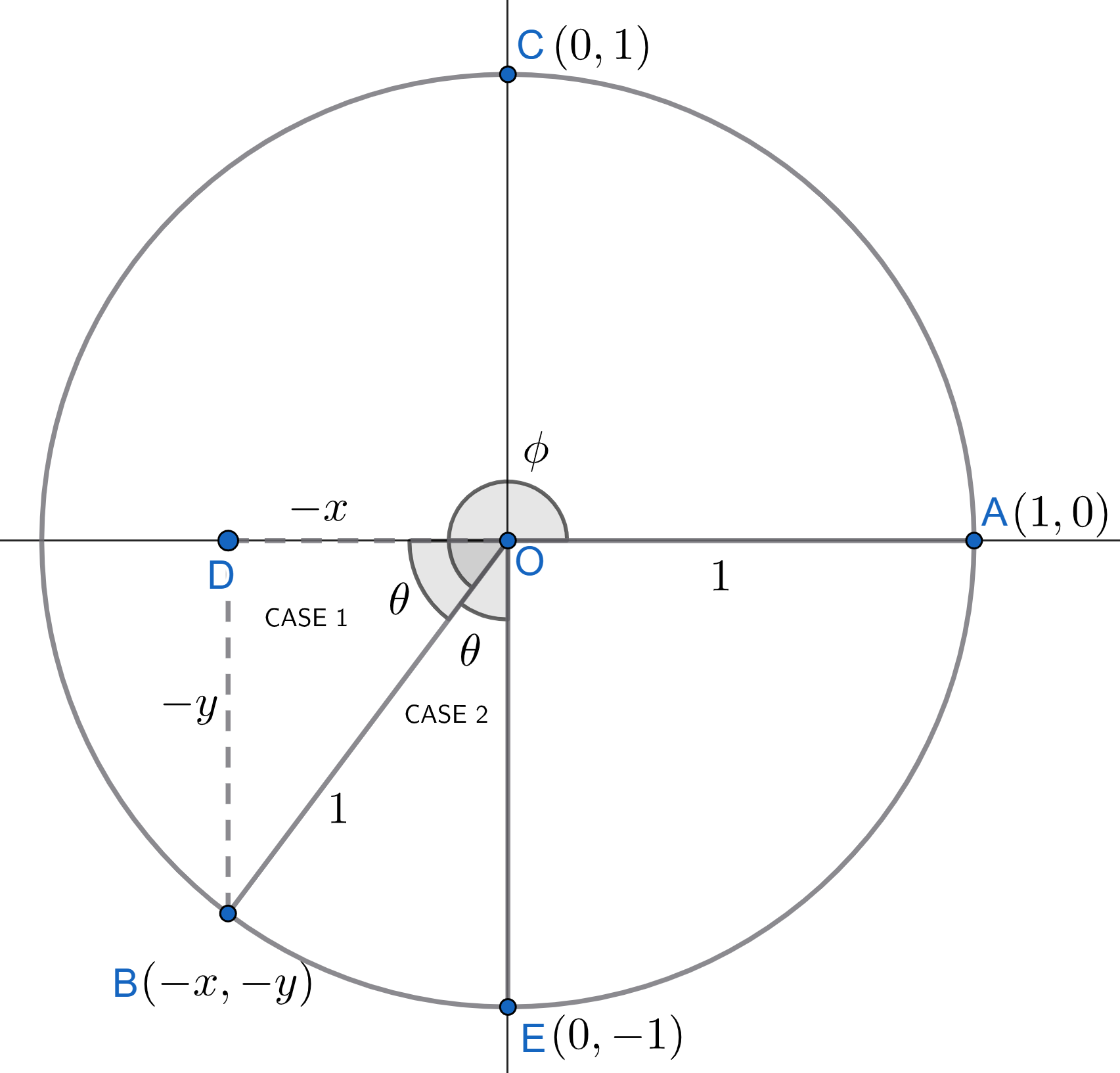
For angles between \(\pi\) and \(3\pi/2\):
The accompanying diagram is shown in figure 2.6.
CASE 1: \((\pi + \theta = \phi)\)
The following relations come out:
$$
\begin{align}
\sin{\left(\pi + \theta\right)} &= -\sin{\theta} \hspace{1cm} \color{red}{(2.13 \text{ i})} \\[4px]
\cos{\left(\pi + \theta\right)} &= -\cos{\theta} \hspace{1cm} \color{red}{(2.13 \text{ ii})} \\[4px]
\tan{\left(\pi + \theta\right)} &= \tan{\theta} \hspace{1cm} \color{red}{(2.13 \text{ iii})} \\[4px]
\csc{\left(\pi + \theta\right)} &= -\csc{\theta} \\[4px]
\sec{\left(\pi + \theta\right)} &= -\sec{\theta} \\[4px]
\cot{\left(\pi + \theta\right)} &= \cot{\theta} \\[4px]
\end{align}
$$
CASE 2: \((\phi + \theta = 3\pi/2)\)
The following relations come out: (see figure)
$$
\begin{align}
\sin{\left(\frac{3\pi}{2} - \theta\right)} &= -\cos{\theta} \hspace{1cm} \color{red}{(2.14 \text{ i})} \\[4px]
\cos{\left(\frac{3\pi}{2} - \theta\right)} &= -\sin{\theta} \hspace{1cm} \color{red}{(2.14 \text{ ii})} \\[4px]
\tan{\left(\frac{3\pi}{2} - \theta\right)} &= \cot{\theta} \hspace{1cm} \color{red}{(2.14 \text{ iii})} \\[4px]
\csc{\left(\frac{3\pi}{2} - \theta\right)} &= -\sec{\theta} \\[4px]
\sec{\left(\frac{3\pi}{2} - \theta\right)} &= -\csc{\theta} \\[4px]
\cot{\left(\frac{3\pi}{2} - \theta\right)} &= \tan{\theta} \\[4px]
\end{align}
$$
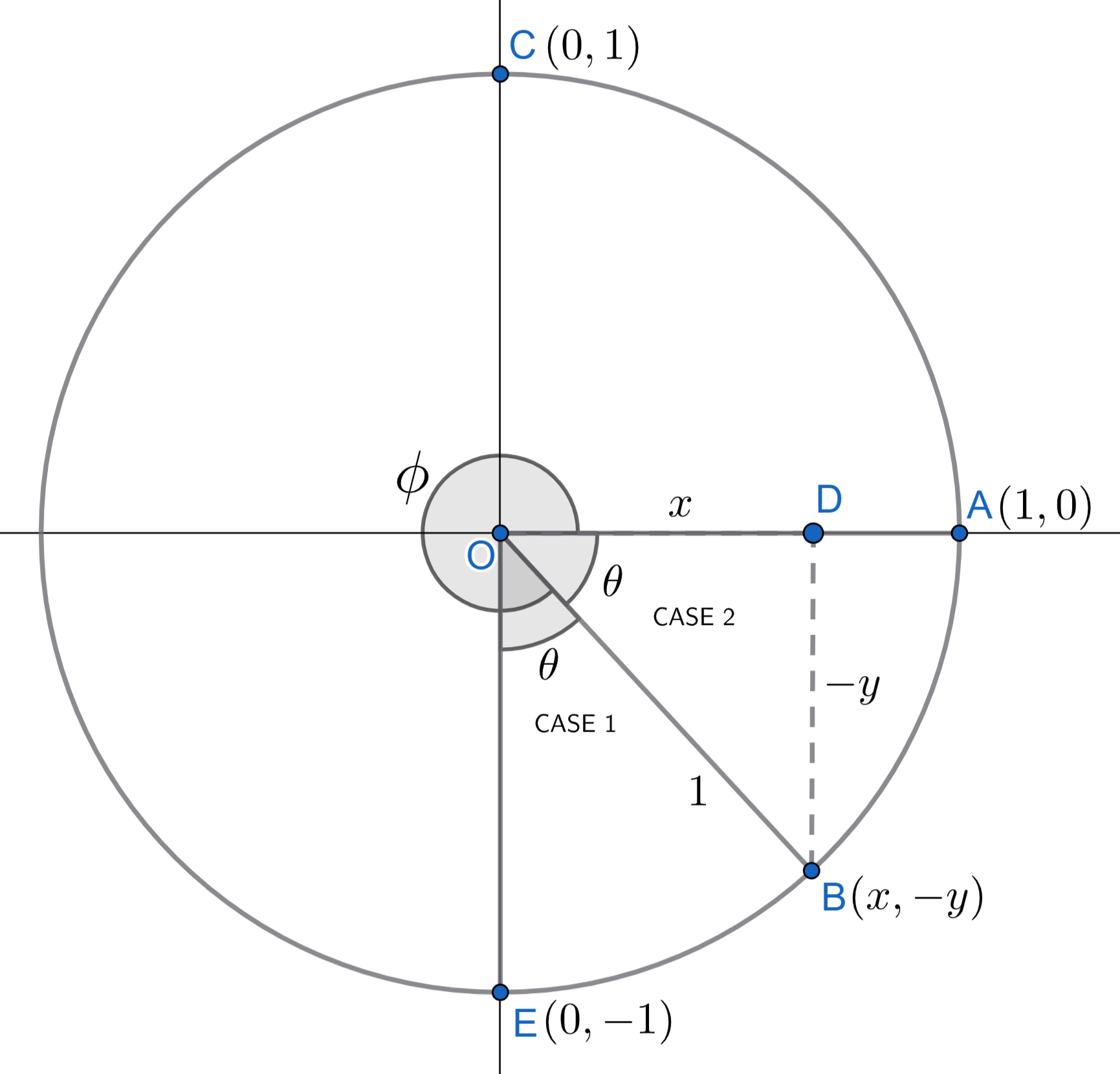
\(\phi\) such that \((3\pi/2 \leq \phi \leq 2\pi)\)
For angles between \(3\pi/2\) and \(2\pi\):
Again, the accompanying diagram is shown in figure 2.7.
CASE 1: \((3\pi/2 + \theta = \phi)\)
The following relations come out:
$$
\begin{align}
\sin{\left(\frac{3\pi}{2} + \theta\right)} &= -\cos{\theta} \hspace{1cm} \color{red}{(2.15\text{ i})} \\[4px]
\cos{\left(\frac{3\pi}{2} + \theta\right)} &= \sin{\theta} \hspace{1cm} \color{red}{(2.15 \text{ ii})} \\[4px]
\tan{\left(\frac{3\pi}{2} + \theta\right)} &= -\cot{\theta} \hspace{1cm} \color{red}{(2.15 \text{ iii})} \\[4px]
\csc{\left(\frac{3\pi}{2} + \theta\right)} &= -\sec{\theta} \\[4px]
\sec{\left(\frac{3\pi}{2} + \theta\right)} &= \csc{\theta} \\[4px]
\cot{\left(\frac{3\pi}{2} + \theta\right)} &= -\tan{\theta} \\[4px]
\end{align}
$$
CASE 2: \((\phi + \theta = 2\pi)\)
The following relations come out: (catch it up from the figure)
$$
\begin{align}
\sin{\left(2\pi - \theta\right)} &= -\sin{\theta} \hspace{1cm} \color{red}{(2.16\text{ i})} \\[4px]
\cos{\left(2\pi - \theta\right)} &= \cos{\theta} \hspace{1cm} \color{red}{(2.16 \text{ ii})} \\[4px]
\tan{\left(2\pi - \theta\right)} &= -\tan{\theta} \hspace{1cm} \color{red}{(2.16 \text{ iii})} \\[4px]
\csc{\left(2\pi - \theta\right)} &= -\csc{\theta} \\[4px]
\sec{\left(2\pi - \theta\right)} &= \sec{\theta} \\[4px]
\cot{\left(2\pi - \theta\right)} &= \cot{\theta} \\[4px]
\end{align}
$$
| Function ↓ \( \theta^{\text{ c}}\) → | \(0\) | \(\pi/6\) | \(\pi/4\) | \(\pi/3\) | \(\pi/2\) | \(2\pi/3\) | \(3\pi/4\) | \(5\pi/6\) | \(\pi\) |
|---|---|---|---|---|---|---|---|---|---|
| \(\sin{\theta}\) | \(0\) | \(1/2\) | \(1/\sqrt{2}\) | \(\sqrt{3}/2\) | \(1\) | \(\sqrt{3}/2\) | \(1/\sqrt{2}\) | \(1/2\) | \(0\) |
| \(\cos{\theta}\) | \(1\) | \(\sqrt{3}/2\) | \(1/\sqrt{2}\) | \(1/2\) | \(0\) | \(-1/2\) | \(-1/\sqrt{2}\) | \(-\sqrt{3}/2\) | \(-1\) |
| \(\tan{\theta}\) | \(0\) | \(1/\sqrt{3}\) | \(1\) | \(\sqrt{3}\) | \(\infty \)* | \(-\sqrt{3}\) | \(-1\) | \(-1/\sqrt{3}\) | \(0\) |
| \(\csc{\theta}\) | \(\infty \) | \(2\) | \(\sqrt{2}\) | \(2/\sqrt{3}\) | \(1\) | \(2/\sqrt{3}\) | \(\sqrt{2}\) | \(2\) | \(\infty\) |
| \(\sec{\theta}\) | \(1\) | \(2/\sqrt{3}\) | \(\sqrt{2}\) | \(2\) | \(\infty \) | \(-2\) | \(-\sqrt{2}\) | \(-2/\sqrt{3}\) | \(-1\) |
| \(\cot{\theta}\) | \(\infty \) | \(\sqrt{3}\) | \(1\) | \(1/\sqrt{3}\) | \(0\) | \(-1/\sqrt{3}\) | \(-1\) | \(-\sqrt{3}\) | \(-\infty\) |
| *here, \(\infty\) represents infinity or undefined | |||||||||
| Function ↓ \( \theta^{\text{ c}}\) → | \(0\) | \(\pi/6\) | \(\pi/4\) | \(\pi/3\) | \(\pi/2\) |
|---|---|---|---|---|---|
| \(\sin{\theta}\) | \(0\) | \(1/2\) | \(1/\sqrt{2}\) | \(\sqrt{3}/2\) | \(1\) |
| \(\cos{\theta}\) | \(1\) | \(\sqrt{3}/2\) | \(1/\sqrt{2}\) | \(1/2\) | \(0\) |
| \(\tan{\theta}\) | \(0\) | \(1/\sqrt{3}\) | \(1\) | \(\sqrt{3}\) | \(\infty \)* |
| \(\csc{\theta}\) | \(\infty \) | \(2\) | \(\sqrt{2}\) | \(2/\sqrt{3}\) | \(1\) |
| \(\sec{\theta}\) | \(1\) | \(2/\sqrt{3}\) | \(\sqrt{2}\) | \(2\) | \(\infty \) |
| \(\cot{\theta}\) | \(\infty \) | \(\sqrt{3}\) | \(1\) | \(1/\sqrt{3}\) | \(0\) |
| *here, \(\infty\) represents infinity or undefined | |||||
| Function ↓ \( \theta^{\text{ c}}\) → | \(2\pi/3\) | \(3\pi/4\) | \(5\pi/6\) | \(\pi\) |
|---|---|---|---|---|
| \(\sin{\theta}\) | \(\sqrt{3}/2\) | \(1/\sqrt{2}\) | \(1/2\) | \(0\) |
| \(\cos{\theta}\) | \(-1/2\) | \(-1/\sqrt{2}\) | \(-\sqrt{3}/2\) | \(-1\) |
| \(\tan{\theta}\) | \(-\sqrt{3}\) | \(-1\) | \(-1/\sqrt{3}\) | \(0\) |
| \(\csc{\theta}\) | \(2/\sqrt{3}\) | \(\sqrt{2}\) | \(2\) | \(\infty\)* |
| \(\sec{\theta}\) | \(-2\) | \(-\sqrt{2}\) | \(-2/\sqrt{3}\) | \(-1\) |
| \(\cot{\theta}\) | \(-1/\sqrt{3}\) | \(-1\) | \(-\sqrt{3}\) | \(-\infty\) |
| *here, \(\infty\) represents infinity or undefined | ||||
So, we have successfully extended our functions from negative acute angles to positive \(2\pi\) radians. To complete the story, we need to say something about the negative obtuse and more smaller angles and about angles above \(2\pi\) radians.
angle case
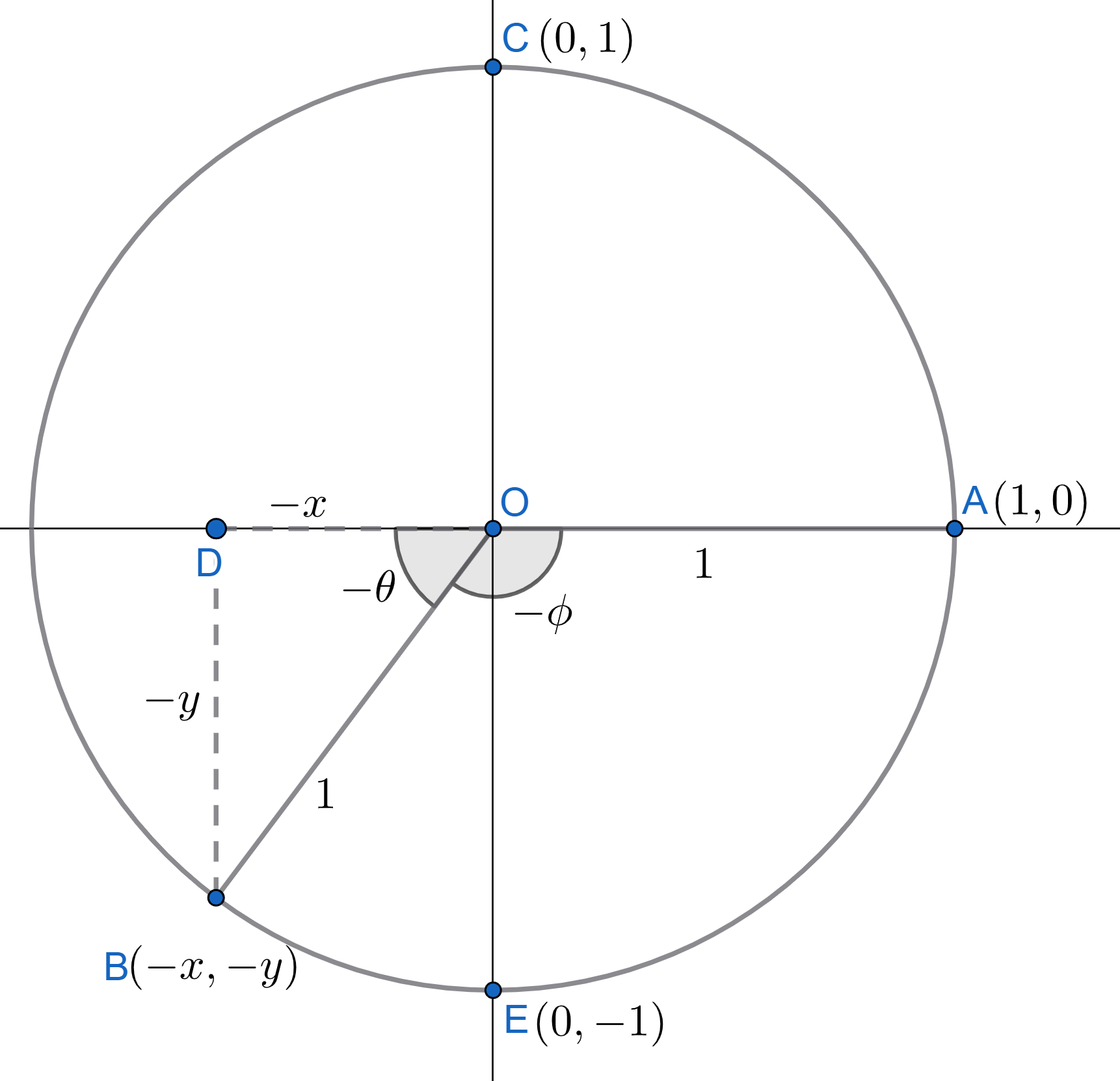
Consider the case of negative obtuse and reflex angles. As we handled the positive obtuse and reflex angles, negatives are handled in the same way with the only difference being the sign. Let's take one example for this :
If there is a negative obtuse angle \(-\phi\) as shown in figure 2.8, with \(-\theta\) completing \(-\pi\) radians i.e. \(-(\phi+\theta) = -\pi\). Then, lets compute the sine of \(-\phi\):
$$
\begin{align}
\sin{(-\phi)} &=\sin{(-\pi-(-\theta))} = \sin{(-(\pi-\theta))} \\[4px]
&= -\sin{(\pi-\theta)} \\[4px]
\sin{(-\phi)} &= -\sin{\theta}
\end{align}
$$
So, in this way we can calculate the functions of negative obtuse angles and reflex angles too, using the same approach as for positive angles,but with appropriate sign adjustments. Pattern can be found in this part too, which is left as exercise to the readers. (Hint: They are similar to the positive angles, if we just account for the negative sign in the beginning using relations eqs 2.10)
But, one question to this theme remains. What about the angles greater than \(2\pi\) and less than \(-2\pi\)? To this we now turn. Consider what would happen in our unit circle picture, when we take an angle, say \((2\pi+ \phi)\), where \(\phi < 2\pi\). Referring to the figure 2.4, the segment OB is just making an angle \(\phi\) with the segment OA, as \(2\pi\) is indicating a \(360^{\circ}\) turn or a complete rotation. Hence, fucntion of any angle beyond \(2\pi\) radians can be written as function of angle less than \(2\pi\), which can be dealt with as in the above sections.
This is similar for negative angles less than \(-2\pi\) radians. We can turn then into angles greater than \(-2\pi\) and then compute them as described above. Let's take an example to compute \(\sin{(2\pi + \pi/6)}\) : $$ \begin{align} \sin{\left(2\pi + \frac{\pi}{6}\right)} &= \sin{\frac{\pi}{6}} = \frac{1}{2} \end{align} $$ Since, \(\pi/6\) represents \(30^{\circ}\).
With this, we have completely extended our trigonometric function's domain to all real numbers. One last thing to emphasize here is that we have been calling the domain to be all real numbers. But, we include angles in the functions as domain. The thing is that the angles are dimensionless quantities and are treated equivalently as simple numbers (this notion is quite useful in Calculus). We have been calling it in angles so as to present its physical picture. Further, it is advisable to think them as this only i.e. in terms of angles and use them as numbers just in calculations.
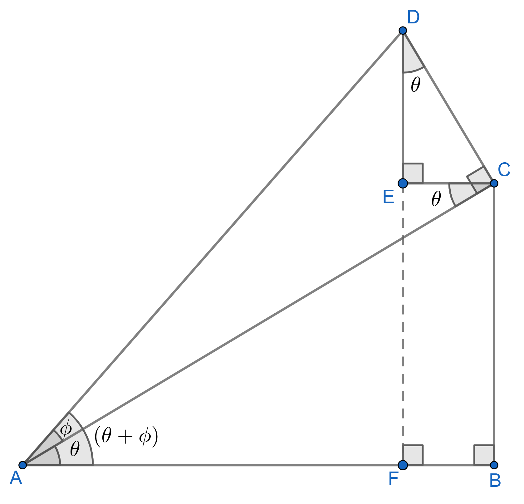
The angle sum relations in trigonometry for a function, relates the function of, say \((\theta + \phi)\) to the function(s) of \(\theta\) and \(\phi\) individually. For example, $$ \sin{(\theta + \phi)} = \sin{\theta}\cos{\phi} + \cos{\theta}\sin{\phi} $$
two distinct angles and their sine
The above relation is one of the angle sum relations. This equation would be our base for building further relations for different function. But, let's see how we get this one in the first place. Consider the figure 2.9 shown.
Here, from the definition of sine, we get: $$ \begin{align} \sin{(\theta + \phi)} &= \frac{DF}{AD} = \frac{DE + EF}{AD} \\[4px] &=\frac{DE}{AD} + \frac{EF}{AD}\\[4px] &= \left(\frac{DE}{DC}\right)\left(\frac{DC}{AD}\right) + \frac{BC}{AD} \end{align} $$
The last step uses the fact that \(EF=BC\). Now, we again use the definitions of sine and cosine in the triangles \(\triangle ABC, \triangle ADC\) and \(\triangle DEC\) to get: $$ \begin{align} \sin{(\theta+\phi)} &= \left(\frac{DE}{DC}\right)\left(\frac{DC}{AD}\right) + \left(\frac{BC}{AC}\right)\left(\frac{AC}{AD}\right) \\[4px] \implies \sin{(\theta+ \phi)} &= \cos{\theta}\sin{\phi} +\sin{\theta}\cos{\phi} \\[4px] \implies \sin{(\theta+ \phi)} &= \sin{\theta}\cos{\phi}+ \cos{\theta}\sin{\phi} \hspace{1cm} \color{red}{(2.17 \text{ i})} \end{align} $$ This proves one of the angle sum relation for sine. For every trigonometric function (sine, cosine and tangent), we would give two relations: one for \((\theta + \phi)\) and other for \((\theta - \phi)\). Though, it is worth mentioning that in regard to remebering these relations, one should at most remember those of sine and cosine and all other can be easily deduced from them.
Above, we derived the expression for \(\sin{(\theta + \phi)}\), now let's see what is \(\sin{(\theta- \phi)}\): $$ \begin{align} \sin{(\theta - \phi)} &= \sin{\left(\theta + (-\phi)\right)} \\[4px] \sin{(\theta - \phi)} &= \sin{\theta}\cos{(-\phi)} + \cos{\theta}\sin{(-\phi)}\\[4px] \sin{(\theta - \phi)} &= \sin{\theta}\cos{\phi} - \cos{\theta}\sin{\phi} \hspace{1cm} (\text{using, eqs 2.10}) \\[4px] & \hspace{5cm} \color{red}{(2.17\text{ ii})} \end{align} $$ In the steps above, we have employed the negative angle property of \(\sin\) and \(\cos\) along with \(\text{eq 2.17 i}\) as indicated. With this, we got our desired relations for sine.
To find \(\cos{(\theta + \phi)}\), we work out as following: $$ \begin{align} \cos{(\theta + \phi)} &= \sin{\left(\frac{\pi}{2}- (\theta + \phi)\right)} \hspace{1cm} (\text{using, eq 2.1 i})\\[4px] &= \sin{\left(\left(\frac{\pi}{2} - \theta\right) + \phi\right)}\\[4px] &= \sin{\left(\frac{\pi}{2} - \theta\right)}\cos{(\phi)} - \cos{\left(\frac{\pi}{2} - \theta\right)}\sin{(\phi)} \\[4px] \cos{(\theta + \phi)} &= \cos{\theta}\cos{\phi} - \sin{\theta}\sin{\phi} \hspace{1cm} \color{red}{\text{(2.18 i)}} \end{align} $$
For moving from last second to the last equation above we again employ \(\text{eq(2.1 i)}\) and \(\text{eq(2.2 i)}\). Further, deriving \(\cos{(\theta - \phi)}\) is the same as was for \(\sin{(\theta - \phi)}\). This is left for the reader as an exercise. The result would be : $$ \cos{(\theta - \phi)} = \cos{\theta}\cos{\phi} + \sin{\theta}\sin{\phi} \hspace{1cm} \color{red}{\text{(2.18 ii)}} $$
To find \(\tan{(\theta + \phi)}\), we go as follows: $$ \begin{align} \tan{(\theta + \phi)} &= \frac{\sin{(\theta + \phi)}}{\cos{(\theta + \phi)}} \\[4px] &= \frac{\sin{\theta}\cos{\phi} + \cos{\theta}\sin{\phi}}{\cos{\theta}\cos{\phi} - \sin{\theta}\sin{\phi}} \\[4px] &= \frac{\frac{\sin{\theta}\cos{\phi} + \cos{\theta}\sin{\phi}}{\cos{\theta}\cos{\phi}}}{\frac{\cos{\theta}\cos{\phi} - \sin{\theta}\sin{\phi}}{\cos{\theta}\cos{\phi}}} \\[4px] \tan{(\theta + \phi)} &= \frac{\tan{\theta} + \tan{\phi}}{1 - \tan{\theta}\tan{\phi}} \hspace{1cm} \color{red}{\text{(2.19 i)}} \end{align} $$ This is the (to say) the most useful form of \(\tan{(\theta + \phi)}\), as it can take many forms as is vivid from the above calculation. Similarly, we can find \(\tan{(\theta - \phi)}\) using the negative angle properties of \(\tan\) (\(\text{eq (2.10 iii)}\)), which again is left as an exercise. The result is mentioned here:
$$ \tan{(\theta - \phi)} = \frac{\tan{\theta} - \tan{\phi}}{1 + \tan{\theta}\tan{\phi}} \hspace{1cm} \color{red}{(2.19 \text{ ii})} $$
Now, for other functions, it can be seen with the help of little algebra that these relations take many forms and those can't be distinguished from each other in terms of simplicity. Also, for cosec and sec, these come rarely and can be dealt with by taking the reciprocal of those of sine and cosine (\(\text{eqs 2.17}\) and \(\text{2.18}\)) respectively. One of them, which should be mentioned is \(\cot{(\theta + \phi)}\): $$ \begin{align} \cot{(\theta + \phi)} &= \frac{1}{\tan{(\theta + \phi)}} \\[4px] &= \frac{1-\tan{\theta}\tan{\phi}}{\tan{\theta} + \tan{\phi}}\\[4px] &= \frac{\frac{1-\tan{\theta}\tan{\phi}}{\tan{\theta}\tan{\phi}}}{\frac{\tan{\theta} + \tan{\phi}}{\tan{\theta}\tan{\phi}}} \\[4px] \cot{(\theta + \phi)} &= \frac{\cot{\theta}\cot{\phi}-1}{\cot{\theta} + \cot{\phi}} \hspace{1cm} \color{red}{\text{(2.20 i)}} \end{align} $$
In a similar way, one can deduce \(\cot{(\theta - \phi)}\) by taking the reciprocal of \(\tan{(\theta - \phi)}\) to get: $$ \cot{(\theta - \phi)} = \frac{\cot{\theta}\cot{\phi} + 1}{\cot{\phi} - \cot{\theta}} \hspace{1cm} \color{red}{\text{(2.20 ii)}} $$
One noticeable thing which turns out here is that, using these relations we can decrease the degree of equations (or trigonometric functions) to linear. This is helpful in integrating trignometric functions of higher orders. One example follows here (can be skipped until calculus section):
Lets perform indefinite integration of \(\sin^2{\theta}\) with respect to \(\theta\): $$ \begin{align} I &= \int{\sin^2{\theta}} \text{ d}\theta \\[4px] I &= \int{\frac{1-\cos{(2\theta)}}{2}} \text{ d}\theta \hspace{1cm} \text{(using, eq (2.22))}\\[4px] I &= \frac{1}{2} \left(\int{\text{d}\theta} - \int{\cos{(2\theta)}}\text{ d}\theta \right) + C\\[4px] I &= \frac{1}{2} \left( \theta - \frac{\sin{(2\theta)}}{2} \right) + C = \frac{\theta}{2} - \frac{\sin{2\theta}}{4} + C \end{align} $$